Divergent transitions in Hilbert Space Gaussian process posteriors and how to avoid them

This builds on research done while in Aki Vehtari’s group at Aalto University, Finland, and is the continuation of a previous blog post, i.e. “Nonparametric statistics: Gaussian processes and their approximations”. This blog post will look at the same dataset and essentially the same model as the previous one, and present a way to maintain much of the promised scalability of Hilbert Space Gaussian Processes (HSGPs), a basis function based approximation to exact Gaussian processes (GPs). Julia (Bezanson et al. (2017)) and Stan (Carpenter et al. (2017)) code is available at https://github.com/generable/public-materials under blog/hsgp-reparam.

‍

1 HSGP primer

HSGPs approximate (non-periodic and 1D in this example) functions f(x) with GP priors via weighted decompositions into mutually orthogonal sine basis functions, i.e.

$$f(x) \approx \frac{1}{L}\sum_{i=1}^m w_i\sin\left(\frac{\pi i}{2L}(\xi(x)+L)\right),$$

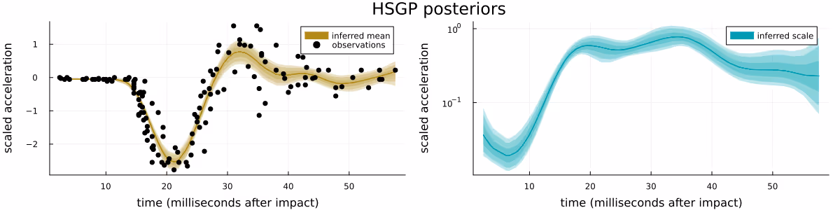
where $L > 1$ is a discretization parameter, $i = 1, \dots, m$ is the basis function number, $m$ is the total number of basis functions, $w_i$ is the weight of the $i$-th basis function (the key unknown parameters), $\xi(x)$ linearly maps $x$ onto $[-1, +1]$, see e.g. Riutort-Mayol et al. (2022) or Solin and Särkkä (2020) for more details. The unknown basis function weights have zero-mean normal priors which depend strongly on the GP hyperparameters, i.e.

$$w_i \sim \mathrm{normal}(0, \sigma^2_\mathrm{GP}\sigma^2_w(\ell_\mathrm{GP}, i)),$$

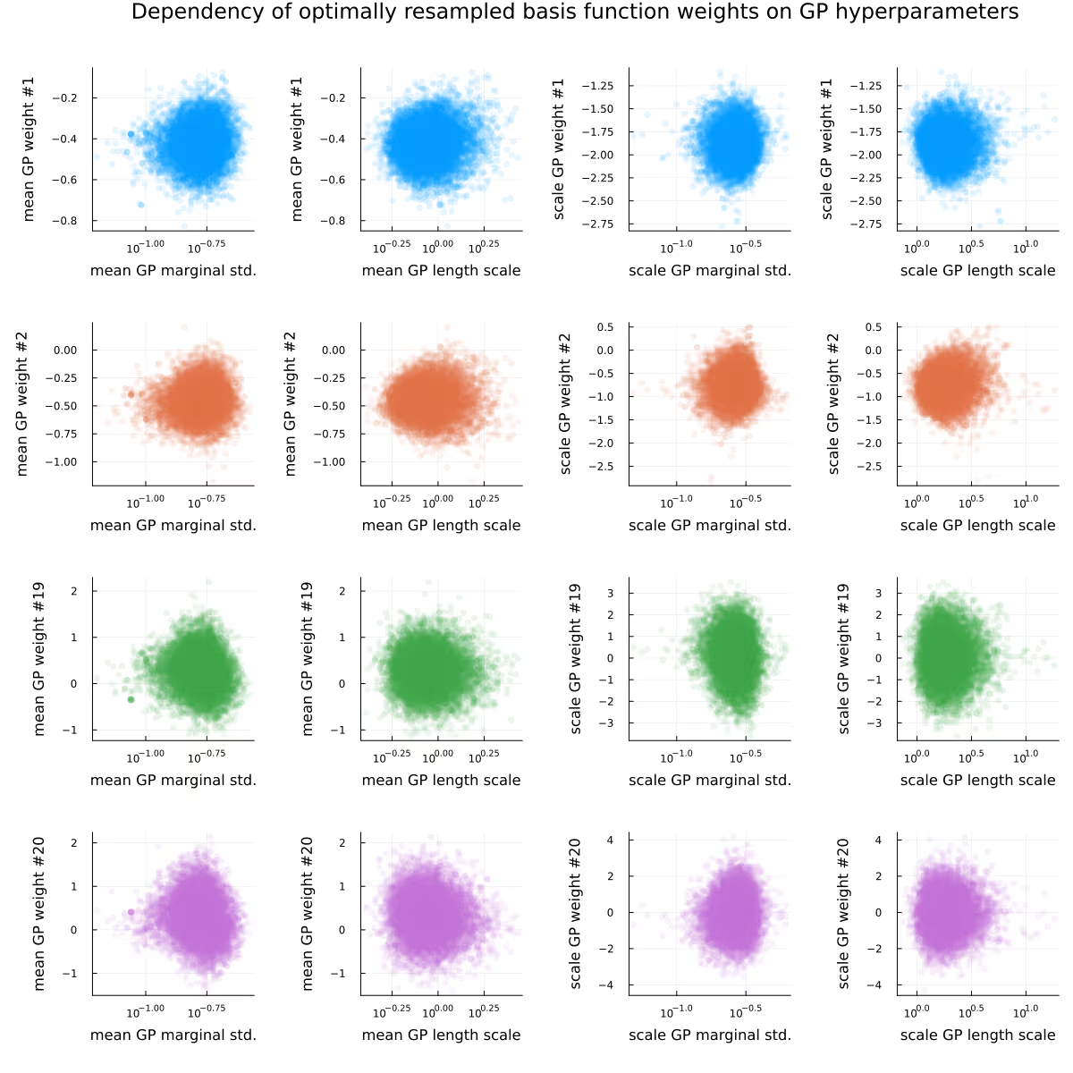
where $\sigma^2_\mathrm{GP}$ is the marginal variance of the GP, $\ell_\mathrm{GP}$ is its length scale, and $\sigma^2_w(\ell_\mathrm{GP}, i)$ is a kernel dependent function. See Figure 1 for a visualization of the basis functions and the dependence of their prior scales on the GP length scale and the basis function number for the used squared exponential kernel.

While this decomposition allows to frontload much of the computational work and to evaluate the approximated function $f(x)$ at $(x_1, \dots, x_n)$ in linear time both in the number of basis functions $m$ and the number of points $n$, the HSGP approximation often gives rise to a posterior geometry which makes the posterior difficult to sample from with standard Markov chain Monte Carlo (MCMC) samplers like the No-U-Turn-Sampler (NUTS). Crucially, as for standard hierarchical models, sampling from HSGP posteriors with standard tools is not as easy as “implement the model once and easily sample from the posteriors due to arbitrary datasets” - instead, different datasets will give rise to different posterior geometries, and will have to be handled differently.

‍

‍

2 HSGP motorcycle posterior

‍

To keep things interesting, we will look again at the heteroscedastic GP model from the previous blog post,

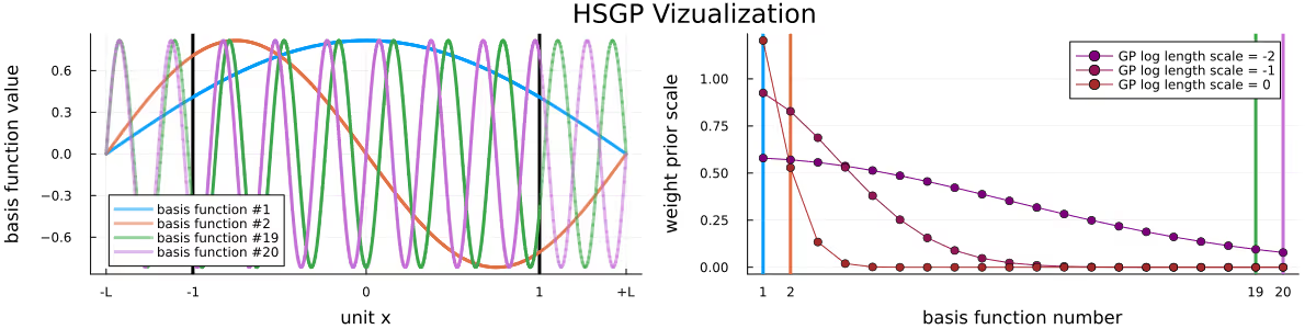
i.e. $y \sim \mathrm{normal}(\mu(x), \exp(\eta(x)))$, $\mu \sim \mathrm{GP}(0, k_\mu)$, and $\eta \sim \mathrm{GP}(0, k_\eta)$ with "appropriate" GP hyperparameter priors (see Section 6.2 for the model implementation), conditioned on the R mcycle dataset, i.e. acceleration data from a simulated motorcycle accident, see Figure 2 for a visualization of the data and the posterior. Similar difficulties are present for easier models such as the corresponding homoscedastic GP model, or more standard hierarchical models, see Section 6.5 in the appendix.

Sampling 10,000 draws using a single chain from that posterior using “Julia’s NUTS” implementation results in a respectable minimal effective sample size (1500), a moderately high average number of leapfrog steps per transition (270), but also a worryingly high fraction of divergent transitions (123 out of 10,000). These divergent transitions are a warning sign indicating potentially inadequate exploration of the posterior in question, and generally show up whenever the posterior exhibits strongly varying local scales. More specifically, they occur whenever the step size of the numerical integrator used by NUTS is too large for parts of the posterior, leading to large Hamiltonian (i.e. total energy) errors and thus to “premature” termination of NUTS’ recursive subtree extension.

Two commonly recommended solutions to this problem of divergent transitions are to reparametrize the model (e.g. switch from a centered parametrization to a non-centered parametrization or vice versa), or to increase the adaptation’s target “acceptance rate” (a slightly misnamed statistic of individual NUTS trajectories) leading to smaller sampling step sizes. Indeed, sometimes finding this good enough parametrization can be easy (e.g. use a centered parametrization for subjects which have a lot of data informing their parameters and use a non-centered parametrization for the ones with little data) and sometimes just waiting “a bit longer” can be feasible. Generally however, finding a “good enough” parametrization can vary wildly in difficulty, and “just” increasing the target acceptance rate is equivalent to throwing more compute at the problem and hoping it goes away - which it might not do.

‍

3 Monolithic non-centered or centered HSGP basis function weights parametrization

So, what even is the problem for this posterior? This is after all no classical hierarchical model, where the issue of a centered or non-centered parametrization directly comes to mind. In fact, there are no "standard" location and scale parameters $\mu$ and $\sigma$ and corresponding hierarchical parameters

$$x_1, \dots, x_n \sim \mathrm{normal}(\mu, \sigma^2).$$

Instead, we have our GP hyperparameters, i.e. the marginal variances $\sigma^2_\mathrm{GP}$ and the length scales $\ell_\mathrm{GP}$ of the two GPs, which, as seen in Section 1 determine the priors on the basis function weights via

$$w_i \sim \mathrm{normal}(0, \sigma^2_\mathrm{GP}\sigma^2_w(\ell_\mathrm{GP}, i)),$$

with (for the used squared exponential kernel)

$$\log(\sigma_w(\ell_\mathrm{GP}, i)) = -\left(\frac{\pi i\ell_\mathrm{GP}}{4L}\right)^2 + \frac{\log(\sqrt{2\pi}\ell_\mathrm{GP})}{2},$$

‍which in fact is more problematic than for the standard hierarchical model as it introduces a much stronger nonlinear dependency between the weight parameters and the hyperparameters. For the sampler, it's an (in the common worst case) double exponential dependence between $\log(\ell_\mathrm{GP})$, the natural "unconstrained"/sampler parametrization of the length scale, and the prior scale $\sigma_w(\ell_\mathrm{GP}, i)$.

To make things worse, the dependence between the GP length scales and the prior scales additionally depends not only on the GPs marginal standard deviation, but also on the basis function number, with the prior scales for higher frequency basis functions depending more strongly on the GP length scales. And finally, in the HSGP setting we are not in the privileged position of the classical hierarchical model of being able to (easily) identify individual weights/parameters with subsets of the data, as all basis functions will couple equally strongly with “all” observations due to the global nature of the basis functions. Generally, it should be such that higher-frequency basis functions will be less strongly identified, while lower-frequency basis function will be more strongly identified, but that’s about all that can generally be said a priori.

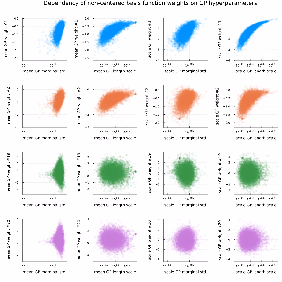
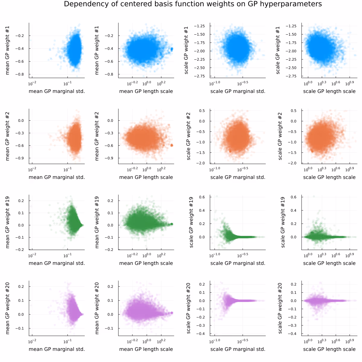
As the conclusion of this section, see Figure 3 and Figure 4, visualizing the posterior dependence of a few basis function weights on the GP hyperparameters for the fully non-centered (Figure 3) and fully centered (Figure 4) parametrization. For both parametrizations, “nonlinear geometries” (i.e. funnels) are visible for some of the basis function weights, as is the usual “sticky” behavior of samples near problematic regions (the “lone” dots visible in the scatter plots).

‍

‍

‍

4 Adaptive HSGP basis function weights parametrization

There has been previous work on the problem of adaptive reparametrizations, including adaptive partial centering, with the main reference being Gorinova, Moore, and Hoffman (2020). The main drawback of that method is maybe that it requires the model to be able to do Variational Inference (VI) on the model and parametrization parameters, something that does not come for free for Stan models. Briefly, the idea of Gorinova, Moore, and Hoffman (2020) is to minimize the KL-divergence $$D_\mathrm{KL}(P || Q) \approx \frac{1}{S}\sum_{s=1}^S\log p(\theta_s) - \log q(\theta_s)$$ of the (reparametrized) posterior $P$ from a (normal) approximation $Q$, which has been convincingly proven to work very well whenever VI works well enough, which it does quite often.

The natural alternative to minimizing the KL-divergence $D_\mathrm{KL}(P || Q)$ of the reparametrized posterior $P$ from a normal approximation $Q$ is just going the other direction, i.e. minimizing the KL-divergence $D_\mathrm{KL}(Q || P)$ of a normal approximation $Q$ from the reparametrized posterior $P$. If the first option is asking “how can we make a normal distribution look as much as possible like the posterior”, then the second option is asking “how can we make the posterior look as much as possible like a normal distribution”, which intuitively seems to be the same question, but has a slightly different answer and also a very different way of being answered.

The main difference between the two options is the samples that are used. In the first option, which we will refer to as the VI-method, we are using samples from the normal approximate distributions to minimize the loss function and find good parametrization parameters, while in the second option, which we will refer to as the MCMC-method, we are using samples from the posterior to minimize the loss function and find good parametrization parameters. Naturally, for the MCMC-method we have the same chicken-and-egg problem as for the learning of the posterior scales (aka as learning of the mass matrix) - without a good guess of the scales (i.e. linear parametrization parameters) or nonlinear parametrization parameters, sampling from the posterior is difficult, but we need good samples from the posterior to obtain a good guess of the linear and nonlinear parametrization parameters.

While this does complicate everything and makes it difficult to have an efficient and robust implementation of the MCMC-method, there’s still hope to have something that works reasonably well and efficiently. In the end, the adaptive reparametrization doesn’t have to be perfect to already help a lot, it just needs to be good enough, and any remaining “imperfactions” in the posterior geometry will have to be solved for better or worse by downstream methods, i.e. by better samplers or by actually using more (but hopefully less than otherwise) compute.

Finally, there are a few ways in which the maths conspire to make the adaptive reparametrization MCMC-method easier to implement and use than could be reasonably expected a priori. Without going into further details here, these are:

• Generally and for “standard” reparametrizations, the “big” (joint) optimization problem decouples into many separate, low-dimensional ones, which are easy to solve separately.
• For each of these separate optimization problems, there is no need to compute anything but the transformed parameters given a candidate parametrization and the jacobian adjustment associated with that reparametrization.
• Given a fixed candidate parametrization, the loss function can be computed “online”, i.e. without holding on to all of the draws that go into the computation of the loss.

Please see Section 6.1 for a Julia implementation of the loss function for the “standard” partially centered parametrization (with zero-mean) of a single hierarchical parameter $w_{(1)}$, i.e. the (re)parametrization

$$w_{(c)} = w_{(0)} \sigma^c \text{ with } w_{(1)} \sim \mathrm{normal}(0, \sigma) \iff w_{(0)} \sim \mathrm{normal}(0, 1).$$

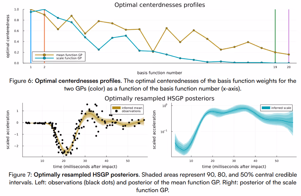
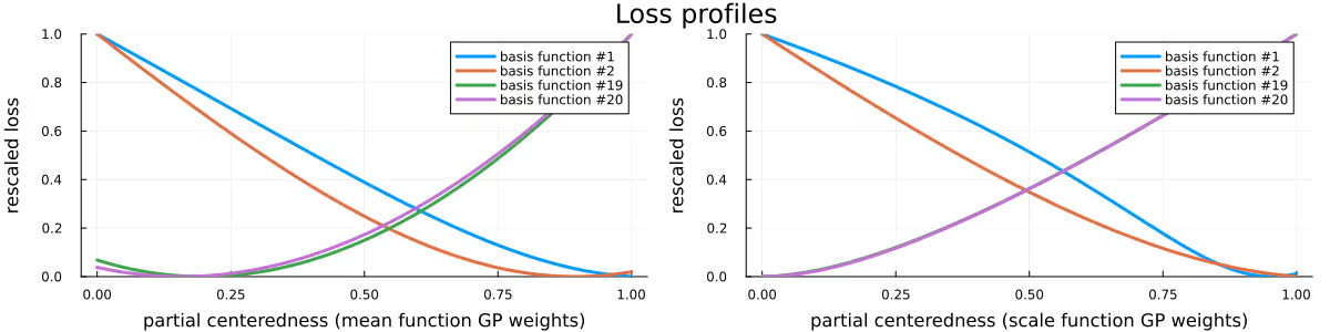
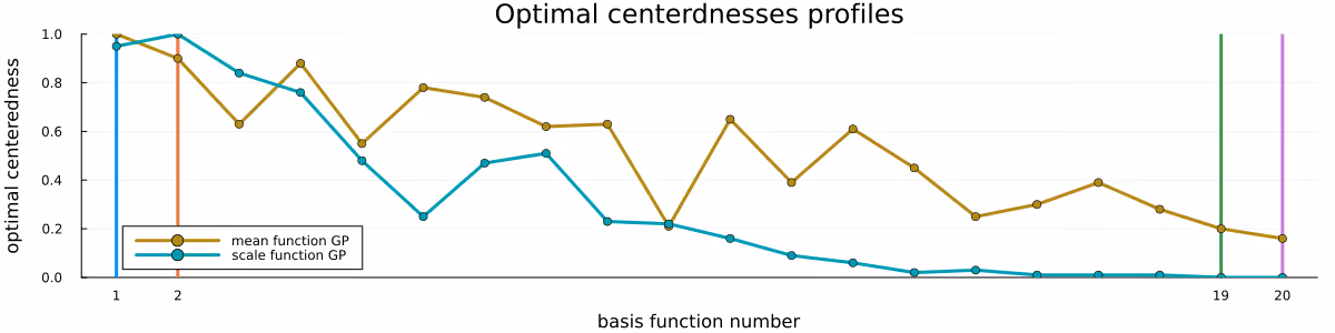
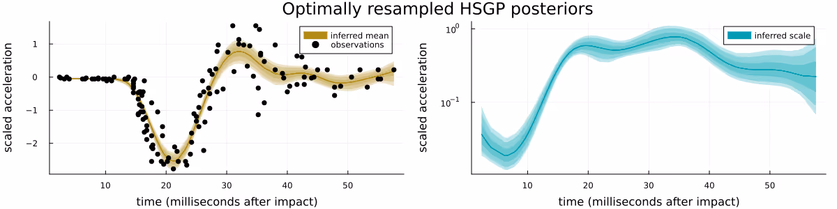
Finally, please see Figure 5 for a visualization of the loss profiles of the MCMC-method for some of the basis function weight parametrizations, Figure 6 for a visualization of the dependence of the optimized partial centeredness on the basis function number (i.e. frequency), Figure 7 for a visualization of the original posterior (as in Figure 2) sampled anew using the optimized parametrization, and Figure 8 for a visualization of the much reduced dependence of the basis function weight parameters on the GP hyperparameters.

Sampling with the optimized parametrization had generally better but not perfect characteristics, specifically we ended up with a higher minimal effective sample (1900 vs 1500), needed fewer average number of leapfrog steps (43 vs 270) and had fewer divergent transitions (35 vs 123 out of 10,000). See also Section 6.4 for a more in-depth comparison.

‍

5 Summary and disclaimers

For this particular set-up we have seen a manifold improvement of sampling efficiency after reparametrization. However, while the reparametrization itself (i.e. parametrization parameters optimization and potentially a transformation of samples) has almost negligible cost, being able to do this reparametrization reliably required us to do an initial sampling run. In principle, it’s possible to combine standard warm-up procedures (which usually learn linear parametrization parameters - the mass matrix) with this optimization of nonlinear parametrization parameters, but doing this both efficiently and reliably in general way is not straightforward.

As done in a previous blog post, some of the free parameters of this case study have been tuned (slightly) to make for a more interesting story and prettier pictures. However, as before, this does not mean that the method presented here is not very often relevant and helpful - in fact, it almost always is. As a matter of fact, the method presented here should (in my opinion) be a standard tool whenever the prior scales of one set of parameters depends on another set of parameters - that is for almost any model. The main drawbacks of the presented method are a) it’s not perfect (but it can help a lot), and b) it requires (minimal) manual effort, both in adapting (Stan) models and in adding some postprocessing to do the reparametrization (something which was handled in a better way in Gorinova, Moore, and Hoffman (2020)).

Finally, a word of caution regarding the use of partially centered parametrizations for HSGP models: Due to the double exponential decay of the basis function weight prior scales, the non-centered parametrization is the only parametrization which does not sometimes-to-often struggle with numerical issues during initialization or sampling. This is because if the basis function weight prior scales underflow to zero, there is no issue for the non-centered parametrization which will just read $w_{(0)} \sim(0, 1); w_{(1)} = 0 w_{(0)}$, but for any partially or fully centered parametrization, which would read $w_{(c)} \sim(0, 0^c); w_{(1)} = 0 w_{(c)}$, evaluation the prior log density of $w_{(c)}$ will return negative infinity and cause a divergence.

‍

References

Bezanson, Jeff, Alan Edelman, Stefan Karpinski, and Viral B. Shah. 2017. “Julia: A Fresh Approach to Numerical Computing.” SIAM Review 59 (1): 65–98. https://doi.org/10.1137/141000671.

Carpenter, Bob, Andrew Gelman, Matthew D. Hoffman, Daniel Lee, Ben Goodrich, Michael Betancourt, Marcus A. Brubaker, Jiqiang Guo, Peter Li, and Allen Riddell. 2017. “Stan: A Probabilistic Programming Language.” Journal of Statistical Software 76: 1. https://doi.org/10.18637/jss.v076.i01.

Gorinova, Maria, Dave Moore, and Matthew Hoffman. 2020. “Automatic Reparameterisation of Probabilistic Programs.” In Proceedings of the 37th International Conference on Machine Learning, 3648–57. PMLR. https://proceedings.mlr.press/v119/gorinova20a.html.

Riutort-Mayol, Gabriel, Paul-Christian Bürkner, Michael R. Andersen, Arno Solin, and Aki Vehtari. 2022. “Practical Hilbert Space Approximate Bayesian Gaussian Processes for Probabilistic Programming.” arXiv. http://arxiv.org/abs/2004.11408.

Solin, Arno, and Simo Särkkä. 2020. “Hilbert Space Methods for Reduced-Rank Gaussian Process Regression.” Statistics and Computing 30 (2): 419–46. https://doi.org/10.1007/s11222-019-09886-w.

‍

6 Appendix

6.1 Loss function Julia implementation

"""
Given posterior draws of

* non-centered parameters (basis function weights in our HSGP example) and
* log scales (usually the scale parameter of the prior of that parameter)

and a candidate centeredness parameter (between 0 and 1), computes the loss function, 
i.e. the KL-divergence of a normal approximation of the reparametrized posterior
from that reparametrized posterior.
"""
loss_function(noncentered_weights::AbstractVector, log_scales::AbstractVector, centerednesses::Real) = begin 
    transformed_weights = noncentered_weights .* exp.(log_scales .* centerednesses)
    log(std(transformed_weights)) - mean(log_scales .* centerednesses)
end

‍

6.2 Standard (non-centered) HSGP Stan implementation

// Generated with [StanBlocks.jl v0.1.5](https://github.com/nsiccha/StanBlocks.jl) via 
functions {
vector normal_lpdfs(
    vector obs,
    vector loc,
    vector scale
) {
    int n = dims(obs)[1];
    return jbroadcasted_normal_lpdfs(obs, loc, scale);
}
vector jbroadcasted_normal_lpdfs(
    vector x1,
    vector x2,
    vector x3
) {
    int n = dims(x1)[1];
    vector[n] rv;
    for(i in 1:n) {
        rv[i] = normal_lpdfs(broadcasted_getindex(x1, i), broadcasted_getindex(x2, i), broadcasted_getindex(x3, i));
    }
    return rv;
}
real normal_lpdfs(
    real args1,
    real args2,
    real args3
) {
    return normal_lpdf(args1 | args2, args3);
}
real broadcasted_getindex(vector x, int i) {
    int m = dims(x)[1];
    return x[i];
}
}
data {
    int x_n;
    vector[x_n] x;
    int n_functions;
    int x_scale_scale;
    int y_scale_scale;
    int y_n;
    vector[y_n] y;
}
transformed data {
    vector[x_n] gp_loc_xi = (-1 + ((2 * (x - min(x))) / (max(x) - min(x))));
    real gp_loc_L = 1.5;
    matrix[x_n, n_functions] gp_loc_X = (
        sin(
            (
                (3.141592653589793 / (2 * gp_loc_L)) *
                (gp_loc_xi + gp_loc_L) *
                (linspaced_vector(n_functions, 1, n_functions)')
            )
        ) /
        sqrt(gp_loc_L)
    );
    vector[x_n] gp_log_scale_xi = (-1 + ((2 * (x - min(x))) / (max(x) - min(x))));
    real gp_log_scale_L = 1.5;
    matrix[x_n, n_functions] gp_log_scale_X = (
        sin(
            (
                (3.141592653589793 / (2 * gp_log_scale_L)) *
                (gp_log_scale_xi + gp_log_scale_L) *
                (linspaced_vector(n_functions, 1, n_functions)')
            )
        ) /
        sqrt(gp_log_scale_L)
    );
}
parameters {
    real gp_loc_log_x_scale;
    real gp_loc_log_y_scale;
    vector[n_functions] gp_loc_unit_weight;
    real gp_log_scale_log_x_scale;
    real gp_log_scale_log_y_scale;
    vector[n_functions] gp_log_scale_unit_weight;
}
transformed parameters {
    real gp_loc_x_scale = exp(gp_loc_log_x_scale);
    vector[n_functions] gp_loc_log_scale = (
        (
            -0.25 *
            (linspaced_vector(n_functions, 1, n_functions) ^ 2) *
            (((gp_loc_x_scale * 3.141592653589793) / (2 * gp_loc_L)) ^ 2)
        ) +
        rep_vector((gp_loc_log_y_scale + 0.45946926660233633 + (0.5 * gp_loc_log_x_scale)), n_functions)
    );
    vector[x_n] gp_loc = (gp_loc_X * (exp(gp_loc_log_scale) .* gp_loc_unit_weight));
    real gp_log_scale_x_scale = exp(gp_log_scale_log_x_scale);
    vector[n_functions] gp_log_scale_log_scale = (
        (
            -0.25 *
            (linspaced_vector(n_functions, 1, n_functions) ^ 2) *
            (((gp_log_scale_x_scale * 3.141592653589793) / (2 * gp_log_scale_L)) ^ 2)
        ) +
        rep_vector(
            (gp_log_scale_log_y_scale + 0.45946926660233633 + (0.5 * gp_log_scale_log_x_scale)),
            n_functions
        )
    );
    vector[x_n] gp_log_scale = (gp_log_scale_X * (exp(gp_log_scale_log_scale) .* gp_log_scale_unit_weight));
}
model {
    gp_loc_log_x_scale ~ normal(0, x_scale_scale);
    gp_loc_log_y_scale ~ normal(0, y_scale_scale);
    gp_loc_unit_weight ~ std_normal();
    gp_log_scale_log_x_scale ~ normal(0, x_scale_scale);
    gp_log_scale_log_y_scale ~ normal(0, y_scale_scale);
    gp_log_scale_unit_weight ~ std_normal();
    y ~ normal(gp_loc, exp(gp_log_scale));
}
generated quantities {
    real gp_loc_y_scale = exp(gp_loc_log_y_scale);
    real gp_log_scale_y_scale = exp(gp_log_scale_log_y_scale);
    vector[y_n] y_likelihood = normal_lpdfs(y, gp_loc, exp(gp_log_scale));
    vector[x_n] y_gen = to_vector(normal_rng(gp_loc, exp(gp_log_scale)));
}

‍

6.3 Partially centered HSGP Stan implementation

// Generated with [StanBlocks.jl v0.1.5](https://github.com/nsiccha/StanBlocks.jl) via 
functions {
vector normal_lpdfs(
    vector obs,
    vector loc,
    vector scale
) {
    int n = dims(obs)[1];
    return jbroadcasted_normal_lpdfs(obs, loc, scale);
}
vector jbroadcasted_normal_lpdfs(
    vector x1,
    vector x2,
    vector x3
) {
    int n = dims(x1)[1];
    vector[n] rv;
    for(i in 1:n) {
        rv[i] = normal_lpdfs(broadcasted_getindex(x1, i), broadcasted_getindex(x2, i), broadcasted_getindex(x3, i));
    }
    return rv;
}
real normal_lpdfs(
    real args1,
    real args2,
    real args3
) {
    return normal_lpdf(args1 | args2, args3);
}
real broadcasted_getindex(vector x, int i) {
    int m = dims(x)[1];
    return x[i];
}
}
data {
    int x_n;
    vector[x_n] x;
    int n_functions;
    int x_scale_scale;
    int y_scale_scale;
    int gp_loc_centerednesses_n;
    vector[gp_loc_centerednesses_n] gp_loc_centerednesses;
    int gp_log_scale_centerednesses_n;
    vector[gp_log_scale_centerednesses_n] gp_log_scale_centerednesses;
    int y_n;
    vector[y_n] y;
}
transformed data {
    vector[x_n] gp_loc_xi = (-1 + ((2 * (x - min(x))) / (max(x) - min(x))));
    real gp_loc_L = 1.5;
    matrix[x_n, n_functions] gp_loc_X = (
        sin(
            (
                (3.141592653589793 / (2 * gp_loc_L)) *
                (gp_loc_xi + gp_loc_L) *
                (linspaced_vector(n_functions, 1, n_functions)')
            )
        ) /
        sqrt(gp_loc_L)
    );
    vector[x_n] gp_log_scale_xi = (-1 + ((2 * (x - min(x))) / (max(x) - min(x))));
    real gp_log_scale_L = 1.5;
    matrix[x_n, n_functions] gp_log_scale_X = (
        sin(
            (
                (3.141592653589793 / (2 * gp_log_scale_L)) *
                (gp_log_scale_xi + gp_log_scale_L) *
                (linspaced_vector(n_functions, 1, n_functions)')
            )
        ) /
        sqrt(gp_log_scale_L)
    );
}
parameters {
    real gp_loc_log_x_scale;
    real gp_loc_log_y_scale;
    vector[n_functions] gp_loc_adaptive_weight;
    real gp_log_scale_log_x_scale;
    real gp_log_scale_log_y_scale;
    vector[n_functions] gp_log_scale_adaptive_weight;
}
transformed parameters {
    real gp_loc_x_scale = exp(gp_loc_log_x_scale);
    vector[n_functions] gp_loc_log_scale = (
        (
            -0.25 *
            (linspaced_vector(n_functions, 1, n_functions) ^ 2) *
            (((gp_loc_x_scale * 3.141592653589793) / (2 * gp_loc_L)) ^ 2)
        ) +
        rep_vector((gp_loc_log_y_scale + 0.45946926660233633 + (0.5 * gp_loc_log_x_scale)), n_functions)
    );
    vector[x_n] gp_loc = (gp_loc_X * (exp((gp_loc_log_scale .* (1 - gp_loc_centerednesses))) .* gp_loc_adaptive_weight));
    real gp_log_scale_x_scale = exp(gp_log_scale_log_x_scale);
    vector[n_functions] gp_log_scale_log_scale = (
        (
            -0.25 *
            (linspaced_vector(n_functions, 1, n_functions) ^ 2) *
            (((gp_log_scale_x_scale * 3.141592653589793) / (2 * gp_log_scale_L)) ^ 2)
        ) +
        rep_vector(
            (gp_log_scale_log_y_scale + 0.45946926660233633 + (0.5 * gp_log_scale_log_x_scale)),
            n_functions
        )
    );
    vector[x_n] gp_log_scale = (
        gp_log_scale_X *
        (exp((gp_log_scale_log_scale .* (1 - gp_log_scale_centerednesses))) .* gp_log_scale_adaptive_weight)
    );
}
model {
    gp_loc_log_x_scale ~ normal(0, x_scale_scale);
    gp_loc_log_y_scale ~ normal(0, y_scale_scale);
    gp_loc_adaptive_weight ~ normal(0, exp((gp_loc_log_scale .* gp_loc_centerednesses)));
    gp_log_scale_log_x_scale ~ normal(0, x_scale_scale);
    gp_log_scale_log_y_scale ~ normal(0, y_scale_scale);
    gp_log_scale_adaptive_weight ~ normal(0, exp((gp_log_scale_log_scale .* gp_log_scale_centerednesses)));
    y ~ normal(gp_loc, exp(gp_log_scale));
}
generated quantities {
    real gp_loc_y_scale = exp(gp_loc_log_y_scale);
    vector[n_functions] gp_loc_unit_weight = (exp(((-gp_loc_log_scale) .* gp_loc_centerednesses)) .* gp_loc_adaptive_weight);
    real gp_log_scale_y_scale = exp(gp_log_scale_log_y_scale);
    vector[n_functions] gp_log_scale_unit_weight = (exp(((-gp_log_scale_log_scale) .* gp_log_scale_centerednesses)) .* gp_log_scale_adaptive_weight);
    vector[y_n] y_likelihood = normal_lpdfs(y, gp_loc, exp(gp_log_scale));
    vector[x_n] y_gen = to_vector(normal_rng(gp_loc, exp(gp_log_scale)));
}

‍

6.4 Sampling statistics comparison (heteroscedastic model)

In the main text, we report sampling statistics for a single long chain with a target acceptance rate of 0.8. Table 1 below reports the same sampling statistics for 40 chains sampling from the heteroscedastic model for varying target acceptance rates (0.8, 0.9 and 0.99).

Table 1: Sampling statistics for the heteroscedastic model. 40 independent chains with 1000 post-warmup draws each are used to sample from the posterior for varying target acceptance rates (left-most column, 0.8, 0.9 and 0.99). We report the minimal ESS (2nd and 5th columns), the total number of gradient evaluations (3rd and 6th columns), and the number of divergences (as “total (histogram over chains)”, 4th and 7th columns) for the non-centered parametrizations (columns 2, 3, and 4) and the partially centered parametrizations (columns 5, 6, and 7). While the individual chains are independent, all partially centered chains use the same optimized parametrization due to the initial long chain from the main text (if apllicable) with 10,000 post warm-up draws.

‍

6.5 Sampling statistics comparison (homoscedastic model)

In the main text, we report sampling statistics for a single long chain for the heteroscedastic model. Table 2 below reports the same sampling statistics for 40 chains sampling from the homoscedastic model for varying target acceptance rates (0.8, 0.9 and 0.99). Generally, due to coupling between the two GPs, sampling from the heteroscedastic model will be more difficult than sampling from the homoscedastic one. Sampling from the homoscedastic model on the other hand will generally be more difficult than sampling from “standard” hierarchical models without shrinkage priors, as the dependence of the prior scales on the GP hyperparameters will usually be stronger. On the other hand, shrinkage priors often lead to even more difficult posterior geometries, because there’s a potentially even stronger interaction between and within different parameter “levels” of the model.

Table 2: Sampling statistics for the homoscedastic model. 40 independent chains with 1000 post-warmup draws each are used to sample from the posterior for varying target acceptance rates (left-most column, 0.8, 0.9 and 0.99). We report the minimal ESS (2nd and 5th columns), the total number of gradient evaluations (3rd and 6th columns), and the number of divergences (as “total (histogram over chains)”, 4th and 7th columns) for the non-centered parametrizations (columns 2, 3, and 4) and the partially centered parametrizations (columns 5, 6, and 7). While the individual chains are independent, all partially centered chains use the same optimized parametrization due to the initial long chain from the main text (if apllicable) with 10,000 post warm-up draws.

For sake of completeness, the two homoscedastic models are also reproduced below.

‍

6.6 Standard (non-centered) HSGP Stan homoscedastic model implementation

// Generated with [StanBlocks.jl v0.1.5](https://github.com/nsiccha/StanBlocks.jl) via 
functions {
vector normal_lpdfs(
    vector obs,
    vector loc,
    real scale
) {
    int n = dims(obs)[1];
    return jbroadcasted_normal_lpdfs(obs, loc, scale);
}
vector jbroadcasted_normal_lpdfs(
    vector x1,
    vector x2,
    real x3
) {
    int n = dims(x1)[1];
    vector[n] rv;
    for(i in 1:n) {
        rv[i] = normal_lpdfs(broadcasted_getindex(x1, i), broadcasted_getindex(x2, i), broadcasted_getindex(x3, i));
    }
    return rv;
}
real normal_lpdfs(
    real args1,
    real args2,
    real args3
) {
    return normal_lpdf(args1 | args2, args3);
}
real broadcasted_getindex(vector x, int i) {
    int m = dims(x)[1];
    return x[i];
}
real broadcasted_getindex(real x, int i) {
    return x;
}
}
data {
    int x_n;
    vector[x_n] x;
    int n_functions;
    int x_scale_scale;
    int y_scale_scale;
    int y_n;
    vector[y_n] y;
}
transformed data {
    vector[x_n] gp_loc_xi = (-1 + ((2 * (x - min(x))) / (max(x) - min(x))));
    real gp_loc_L = 1.5;
    matrix[x_n, n_functions] gp_loc_X = (
        sin(
            (
                (3.141592653589793 / (2 * gp_loc_L)) *
                (gp_loc_xi + gp_loc_L) *
                (linspaced_vector(n_functions, 1, n_functions)')
            )
        ) /
        sqrt(gp_loc_L)
    );
}
parameters {
    real gp_loc_log_x_scale;
    real gp_loc_log_y_scale;
    vector[n_functions] gp_loc_unit_weight;
    real gp_log_scale;
}
transformed parameters {
    real gp_loc_x_scale = exp(gp_loc_log_x_scale);
    vector[n_functions] gp_loc_log_scale = (
        (
            -0.25 *
            (linspaced_vector(n_functions, 1, n_functions) ^ 2) *
            (((gp_loc_x_scale * 3.141592653589793) / (2 * gp_loc_L)) ^ 2)
        ) +
        rep_vector((gp_loc_log_y_scale + 0.45946926660233633 + (0.5 * gp_loc_log_x_scale)), n_functions)
    );
    vector[x_n] gp_loc = (gp_loc_X * (exp(gp_loc_log_scale) .* gp_loc_unit_weight));
}
model {
    gp_loc_log_x_scale ~ normal(0, x_scale_scale);
    gp_loc_log_y_scale ~ normal(0, y_scale_scale);
    gp_loc_unit_weight ~ std_normal();
    gp_log_scale ~ normal(0, y_scale_scale);
    y ~ normal(gp_loc, exp(gp_log_scale));
}
generated quantities {
    real gp_loc_y_scale = exp(gp_loc_log_y_scale);
    vector[y_n] y_likelihood = normal_lpdfs(y, gp_loc, exp(gp_log_scale));
    vector[x_n] y_gen = to_vector(normal_rng(gp_loc, exp(gp_log_scale)));
}

‍

6.7 Partially centered HSGP Stan homoscedastic model implementation

// Generated with [StanBlocks.jl v0.1.5](https://github.com/nsiccha/StanBlocks.jl) via 
functions {
vector normal_lpdfs(
    vector obs,
    vector loc,
    real scale
) {
    int n = dims(obs)[1];
    return jbroadcasted_normal_lpdfs(obs, loc, scale);
}
vector jbroadcasted_normal_lpdfs(
    vector x1,
    vector x2,
    real x3
) {
    int n = dims(x1)[1];
    vector[n] rv;
    for(i in 1:n) {
        rv[i] = normal_lpdfs(broadcasted_getindex(x1, i), broadcasted_getindex(x2, i), broadcasted_getindex(x3, i));
    }
    return rv;
}
real normal_lpdfs(
    real args1,
    real args2,
    real args3
) {
    return normal_lpdf(args1 | args2, args3);
}
real broadcasted_getindex(vector x, int i) {
    int m = dims(x)[1];
    return x[i];
}
real broadcasted_getindex(real x, int i) {
    return x;
}
}
data {
    int x_n;
    vector[x_n] x;
    int n_functions;
    int x_scale_scale;
    int y_scale_scale;
    int gp_loc_centerednesses_n;
    vector[gp_loc_centerednesses_n] gp_loc_centerednesses;
    int y_n;
    vector[y_n] y;
}
transformed data {
    vector[x_n] gp_loc_xi = (-1 + ((2 * (x - min(x))) / (max(x) - min(x))));
    real gp_loc_L = 1.5;
    matrix[x_n, n_functions] gp_loc_X = (
        sin(
            (
                (3.141592653589793 / (2 * gp_loc_L)) *
                (gp_loc_xi + gp_loc_L) *
                (linspaced_vector(n_functions, 1, n_functions)')
            )
        ) /
        sqrt(gp_loc_L)
    );
}
parameters {
    real gp_loc_log_x_scale;
    real gp_loc_log_y_scale;
    vector[n_functions] gp_loc_adaptive_weight;
    real gp_log_scale;
}
transformed parameters {
    real gp_loc_x_scale = exp(gp_loc_log_x_scale);
    vector[n_functions] gp_loc_log_scale = (
        (
            -0.25 *
            (linspaced_vector(n_functions, 1, n_functions) ^ 2) *
            (((gp_loc_x_scale * 3.141592653589793) / (2 * gp_loc_L)) ^ 2)
        ) +
        rep_vector((gp_loc_log_y_scale + 0.45946926660233633 + (0.5 * gp_loc_log_x_scale)), n_functions)
    );
    vector[x_n] gp_loc = (gp_loc_X * (exp((gp_loc_log_scale .* (1 - gp_loc_centerednesses))) .* gp_loc_adaptive_weight));
}
model {
    gp_loc_log_x_scale ~ normal(0, x_scale_scale);
    gp_loc_log_y_scale ~ normal(0, y_scale_scale);
    gp_loc_adaptive_weight ~ normal(0, exp((gp_loc_log_scale .* gp_loc_centerednesses)));
    gp_log_scale ~ normal(0, y_scale_scale);
    y ~ normal(gp_loc, exp(gp_log_scale));
}
generated quantities {
    real gp_loc_y_scale = exp(gp_loc_log_y_scale);
    vector[n_functions] gp_loc_unit_weight = (exp(((-gp_loc_log_scale) .* gp_loc_centerednesses)) .* gp_loc_adaptive_weight);
    vector[y_n] y_likelihood = normal_lpdfs(y, gp_loc, exp(gp_log_scale));
    vector[x_n] y_gen = to_vector(normal_rng(gp_loc, exp(gp_log_scale)));
}

‍