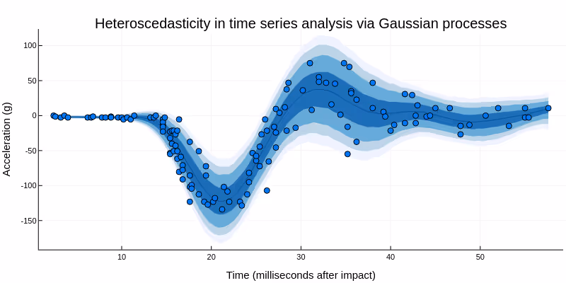
Nonparametric statistics: Gaussian processes and their approximations

The promise of Gaussian processes

Nonparametric statistical model components are a flexible tool for imposing structure on observable or latent processes. Usually, nonparametric statistical models have an uncountably infinite number of free parameters, but reduce their effective flexibility by constraining these parameters to covary in ways that guard against overfitting.

Gaussian processes represent one family of such models. Mathematically, putting a Gaussian process prior with mean function $\mu$ and covariance function $k$ on a function $f$, i.e.

$$f \sim \mathrm{GP}(\mu, k),$$

implies that for any $x_1$ and $x_2$, the joint prior distribution of $f(x_1)$ and $f(x_2)$ is a multivariate Gaussian distribution with mean $[\mu(x_1), \mu(x_2)]^T$ and covariance $k(x_1, x_2)$. The mean function $\mu$ can be as simple as a constant value (e.g. $\mu(x) = 0$), but often depends on other model parameters and covariates. Common choices for the covariance function $k$ include:

• the squared exponential function, which imposes very strong regularity on the function $f$, and
• the Matérn family of covariance functions, which allows to vary the imposed regularity.

For an interactive visualization of different combinations of kernel functions, hyperparameters, and observations, see Ti John’s excellent Interactive Gaussian process Visualization.

By wrapping the function $f$ in appropriate link functions, which may in turn depend on other model parameters or covariates, Gaussian processes allow the modeler both to "let the data speak for itself" and to impose prior beliefs on the modelled function $f$. For example:

• with covariates $x$ and observations $y$, you get heteroscedasticity via an observation model $y \sim \mathrm{Normal}(\mu(x), \exp(\eta(x)))$ with $\mu \sim \mathrm{GP}(0, k_\mu)$ and $\eta \sim \mathrm{GP}(0, k_\eta)$, visualized below for acceleration data from a simulated motorcycle accident, or
• with temporospatial covariates $x$, $y$ and count data $n$, you get a log Gaussian Cox process via an observation model $n \sim \mathrm{Poisson}(\exp(\mu(x, y)))$ with $\mu \sim \mathrm{GP}(0, k_\mu)$.

‍

‍

A challenge with Gaussian processes - the choice of hyperprior

Every Gaussian process comes with a set of "tunable" or inferrable hyperparameters. In the field of machine learning, these hyperparameters are usually optimized and then fixed for further inference. While this approach often works very well in the "big data" setting typical of machine learning, with health data, we are often left with less data than we would like, but still have to reach robust conclusions and make high-stakes decisions. To do so, we must properly account for any relevant residual uncertainty, which regularly includes the choice of hyperparameters for the covariance functions $k$.

For a function $f \sim \mathrm{GP}(\mu, k)$ depending on a single covariate $x$, and with the covariance function $k$ being the squared exponential function, there are two positive hyperparameters:

• the marginal variance $\sigma^2$, affecting the typical variance around the mean function $\mu$, and
• the length scale $\ell$, affecting the "wiggliness" of $f$.

Without previous experience, it can be exceedingly difficult to specify principled priors for these hyperparameters. Poorly chosen priors can, in turn, substantially affect final conclusions and decisions.

‍

The problem with Gaussian processes - unfortunate scaling

Even after settling on a covariance function and hyperpriors, there remains the issue of scaling.

For exact Gaussian process regression with variable hyperparameters, computing the prior density has cubic complexity in the number of distinct observation points. This means that evaluating the prior or posterior density even for the simplest possible model $y \sim \mathrm{Normal}(\mu(x), \sigma^2)$ with $\mu \sim \mathrm{GP}(0, k)$ will take 8 times as long if you double the number of distinct values of the covariate $x$. This happens because, under the hood, to evaluate the prior density of $\mu(x) \sim \mathrm{Normal}(0, \Sigma)$ for $n$ distinct covariate values $x$, we have to first construct the full covariance matrix $\Sigma$ and then perform its Cholesky decomposition, which has the cubic complexity in $n$.

Scaling quickly becomes prohibitive if the hyperparameters are allowed to vary - which as discussed previously is often a prerequisite to making robust decisions under uncertainty. After all, "full" Bayesian inference, as realized through the use of Markov Chain Monte Carlo methods, often requires evaluating the posterior log density and its gradient many thousands to millions of times. Even fixing the hyperparameters will only reduce the scaling from cubic to effectively quadratic, because while fixed hyperparameters allow the Cholesky decomposition to be precomputed and reused, we will still have to multiply with or divide by it at every posterior log density evaluation.

Fortunately, there are solutions, which however come with their own challenges.

‍

Practical approximations to Gaussian processes

There are two main ways to discretize Gaussian processes, both of which use a finite number $m$ of basis functions $\phi_i$ to approximate a function $f \sim \mathrm{GP}(0, k)$ as

$$f(x) \approx \sum_{i=1}^m w_i \phi_i(x):$$

• The inducing points approximation chooses $\phi_i(x) = k(x_i, x)$, where $x_i$ are the eponymous inducing points. For fixed hyperparameters, the matrix of values of the basis functions at the covariate values $x$ can be precomputed and the basis function weights $w_i$ have a multivariate Gaussian prior, making this discretization a popular choice in machine learning.
• The Hilbert space approximation instead uses scaled and shifted sine waves of varying frequencies, i.e. $\phi_i(x) = c_1\sin(\lambda_i(x+c_2))$ with $c_1$ and $c_2$ approximation dependent constants, and $\lambda_i$ kernel function dependent but hyperparameter independent and thus precomputable positive numbers. For both fixed and variable hyperparameters, the matrix of values of the basis functions at the covariate values $x$ can be precomputed.

Both approximations eliminate the at least quadratic complexity in the number $n$ of distinct covariate values $x$, if the number $m$ of basis functions does not depend on $n$:

• The inducing points approximation trades in the cubic complexity in $n$ for cubic complexity in $m$, which can be more than good enough if $m \lll n$, and which lowers to effectively quadratic if the hyperparameters are fixed and the needed "smaller" Cholesky decomposition can be frontloaded.
• The Hilbert space approximation does not require any Cholesky decomposition, and thus scales linearly in both $m$ and $n$, effectively reducing the evaluation of the Gaussian process prior to a simple dense matrix-vector product.

The main benefit of the inducing points approximation over the Hilbert space approximation is due to the locality of the basis functions of the inducing point approximation: If you only need to approximate your Gaussian process in small and potentially disjointed subsets of its underlying covariate space, the inducing point approximation allows you to only allocate basis functions to these subsets, which is something that the Hilbert space approximation is incapable of, as its basis functions are fully "global". This can be particularly noteworthy in higher-dimensional covariate spaces, where the "full" Hilbert space approximation always scales exponentially with the dimension, while the inducing points approximation potentially does not. In practice however, this advantage seldomly materializes, and there are good alternatives to the "full" Hilbert space approximation such as additive Gaussian processes as implemented in Juho's `lgpr` package.

‍

Impractical problems for otherwise practical approximations to Gaussian processes

Generally, because we want to propagate the uncertainty about the hyperparameters and thus will not fix them, we are using the Hilbert space Gaussian process approximation at Generable. However, even though the scaling of this approximation is linear and thus optimal when considering only the cost of evaluating a single posterior log density, making use of it in practice can often be quite challenging. Specifically, it is common to observe much worse than linear scaling in the number of observations if the approximation is used naively. The root of this problem lies in the oft-quoted specter of "bad" or "inappropriate" parametrizations, and does also affect both the exact Gaussian process regression and its approximation via inducing points.

We will revisit this problem and its solution in a later post in this series.

‍

‍

‍

‍