

Just a while ago, I was at a conference where someone was trying to fit complicated ODE models in Stan and struggling with the computational difficulty. It is not uncommon to see sampling issues with these models, and I think many of the problems stem from applying classic numerical analysis methods to a context for which they were not designed.
Let's say you have a model and want to evaluate the likelihood given parameters $\theta$ at, say, $\theta = 2.1$. How accurate is the result that you get on your computer? How does the error propagate to your final inferences?
Of course, the first issue is that many values like $2.1$ cannot be exactly represented since there is only a finite set of possible binary representations with a given number of bits. Suppose you are using 64-bit floating point numbers with the IEEE 754 standard. The unit round-off, i.e., the maximum relative error you can get when rounding a real number to the nearest floating-point number, in this case is I think something like $u \approx 1.1 \cdot 10^{-16}$. Also, your likelihood formula probably consists of many elementary operations, each of which contributing to the final error.
In the above example, the round-off error in the likelihood is likely still relatively small if the implementation is well-conditioned and avoids underflow/overflow. So, for the remainder of this post, I ignore the error due to finite-precision floating-point representation and focus on a different numerical issue that persists even if we had infinite-precision floats. I am referring to the case when the likelihood depends on some intermediate quantity $y(\theta)$ for which you don't have a closed-form formula, and you have to approximate it using a numerical solver. The classic example is nonlinear ordinary differential equation (ODE) initial value problems (IVPs).
ODE example
For demonstration, I use a linear ODE example to compare the likelihood obtained from the true closed-form IVP solution with that from a numerical solver. Consider the one-compartment pharmacokinetic system
$$
\begin{cases}\frac{\text{d}}{\text{d}t}y_1 &= -k_a \cdot y_1 \\\frac{\text{d}}{\text{d}t}y_2 &= k_a \cdot y_1 - k_e \cdot y_2,\end{cases}
$$
where $y_1$, $y_2$ denote the mass of drug in the depot and central compartments, respectively, and $k_a$, $k_e$ are the absorption and elimination rates. Now if a dose $D$ is given at time $t=0$, this gives us an IVP with $y_1(0) = D$, $y_2(0) = 0$. It has the closed-form solution
$$
y_2(t)= D \frac{k_a}{k_a - k_e} \left( e^{-k_e t} - e^{-k_a t} \right)
$$
and the concentration in the central compartment is $C(t) = \frac{y_2(t)}{V}$, where I fix the volume of the central compartment $V = 30$ L.
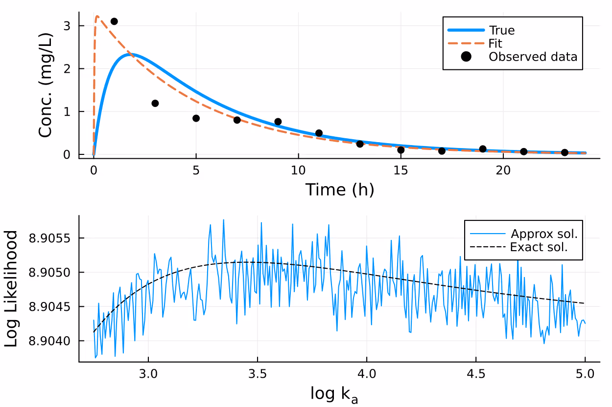
Seen in the upper panel of the figure below is log-normally distributed data around the true concentration $C(t)$, simulated with $D = 100$ mg, $k_e = 0.2$ 1/h and $k_a = 1.2$ 1/h. In the lower panel, I fix all other parameters to their true values and study the likelihood as a function of $k_a$. Interestingly, for this data realization, the maximum likelihood is obtained with a very high $k_a \approx e^{3.4}$. This maximum likelihood fit is shown in the upper panel, with the orange dashed line.
The jagged blue line is the likelihood profile that I get using the adaptive Tsitouras 5/4 solver in Julia, with absolute and relative tolerance $\epsilon = 10^{-3}$. Now, imagine you are an MCMC sampler trying to explore this likelihood surface! These jagged likelihood surfaces, which are solely artifacts of the numerical procedures, have been reported by others; I recommend the article [1] for more information and examples.
Adaptive ODE solvers try to estimate their own local truncation error (LTE), i.e., the error caused by a single internal step, and adapt their step size during integration so that the estimated $\hat{\mathrm{LTE}}$ satisfies some tolerances. The step size update rules in implementations of popular adaptive solvers are typically roughly of the form
$$
\begin{cases}
\text{if } \hat{\mathrm{LTE}} > A &\text{reject step and decrease step size} \\
\text{if } B \leq \hat{\mathrm{LTE}} \leq A &\text{accept step and keep same step size} \\
\text{if } \hat{\mathrm{LTE}} < B &\text{accept step and increase step size}\end{cases}
$$
where $A, B$ are suitable values derived based on the given tolerances. Different $\theta$ can require a different number of steps to satisfy the adaptation rules, so numerical solutions, and therefore the corresponding likelihood, change discontinuously with respect to $\theta$.
When using these solvers with MCMC, one should run the inference many times, each time tightening the tolerances until the results stop changing. However, this is computationally painful, since
Niko and I are authors of a paper [2] in which we studied these issues and developed an improved strategy based on importance sampling. We highlight that a fixed-step-size solver approach becomes attractive because it avoids the jaggedness issue and the gradient mismatch problem that adaptive solvers introduce. Also, failure with a too large step size is usually fast in this case. Error control of the ODE solution is not really needed if we are going to do the inference reruns with smaller and smaller step sizes anyway.
We once considered whether it would be possible to design an adaptive solver with a continuous adaptation rule. This would eliminate the jaggedness problem and, when used with the gradual tolerance tightening scheme, could retain the reliability of the inferences.
There also exists a field called probabilistic numerics. Probabilistic ODE solvers such as the ones in ProbNumDiffEq.jl estimate a probability distribution over the solver error. This is a field I am less familiar with. In my understanding, such solvers could be used with MCMC so that each the likelihood evaluation at some $\theta$ is a marginal likelihood integrated over the solver error distribution at $\theta$. These methods don't seem to have been widely adopted and have not been implemented in for example Stan.
One idea, which also [1] suggested, is to perform error control on the likelihood rather than the ODE solution. However, this cannot be done in something like Stan. Ultimately, what we would really want is error control on the final inferences (expectations), but that is even further away.
[1] Creswell R, Shepherd KM, Lambert B, Mirams GR, Lei CL, Tavener S, Robinson M, Gavaghan DJ. Understanding the impact of numerical solvers on inference for differential equation models. J R Soc Interface. 2024 Mar;21(212):20230369. doi: 10.1098/rsif.2023.0369.
[2] Timonen, J., Siccha, N., Bales, B., Lähdesmäki, H., & Vehtari, A. (2023). An importance sampling approach for reliable and efficient inference in Bayesian ordinary differential equation models. Stat, 12(1), e614. https://doi.org/10.1002/sta4.614
This is a comment related to the post above. It was submitted in a form, formatted by Make, and then approved by an admin. After getting approved, it was sent to Webflow and stored in a rich text field.
This is a comment related to the post above. It was submitted in a form, formatted by Make, and then approved by an admin. After getting approved, it was sent to Webflow and stored in a rich text field.
This is a comment related to the post above. It was submitted in a form, formatted by Make, and then approved by an admin. After getting approved, it was sent to Webflow and stored in a rich text field.
This is a comment related to the post above. It was submitted in a form, formatted by Make, and then approved by an admin. After getting approved, it was sent to Webflow and stored in a rich text field.
This is a comment related to the post above. It was submitted in a form, formatted by Make, and then approved by an admin. After getting approved, it was sent to Webflow and stored in a rich text field.
This is a comment related to the post above. It was submitted in a form, formatted by Make, and then approved by an admin. After getting approved, it was sent to Webflow and stored in a rich text field.
This is a comment related to the post above. It was submitted in a form, formatted by Make, and then approved by an admin. After getting approved, it was sent to Webflow and stored in a rich text field.
This is a comment related to the post above. It was submitted in a form, formatted by Make, and then approved by an admin. After getting approved, it was sent to Webflow and stored in a rich text field.
This is a comment related to the post above. It was submitted in a form, formatted by Make, and then approved by an admin. After getting approved, it was sent to Webflow and stored in a rich text field.
This is a comment related to the post above. It was submitted in a form, formatted by Make, and then approved by an admin. After getting approved, it was sent to Webflow and stored in a rich text field.
This is a comment related to the post above. It was submitted in a form, formatted by Make, and then approved by an admin. After getting approved, it was sent to Webflow and stored in a rich text field.
This is a comment related to the post above. It was submitted in a form, formatted by Make, and then approved by an admin. After getting approved, it was sent to Webflow and stored in a rich text field.
This is a comment related to the post above. It was submitted in a form, formatted by Make, and then approved by an admin. After getting approved, it was sent to Webflow and stored in a rich text field.
This is a comment related to the post above. It was submitted in a form, formatted by Make, and then approved by an admin. After getting approved, it was sent to Webflow and stored in a rich text field.
This is a comment related to the post above. It was submitted in a form, formatted by Make, and then approved by an admin. After getting approved, it was sent to Webflow and stored in a rich text field.
This is a comment related to the post above. It was submitted in a form, formatted by Make, and then approved by an admin. After getting approved, it was sent to Webflow and stored in a rich text field.
This is a comment related to the post above. It was submitted in a form, formatted by Make, and then approved by an admin. After getting approved, it was sent to Webflow and stored in a rich text field.
This is a comment related to the post above. It was submitted in a form, formatted by Make, and then approved by an admin. After getting approved, it was sent to Webflow and stored in a rich text field.
This is a comment related to the post above. It was submitted in a form, formatted by Make, and then approved by an admin. After getting approved, it was sent to Webflow and stored in a rich text field.
This is a comment related to the post above. It was submitted in a form, formatted by Make, and then approved by an admin. After getting approved, it was sent to Webflow and stored in a rich text field.
This is a comment related to the post above. It was submitted in a form, formatted by Make, and then approved by an admin. After getting approved, it was sent to Webflow and stored in a rich text field.
This is a comment related to the post above. It was submitted in a form, formatted by Make, and then approved by an admin. After getting approved, it was sent to Webflow and stored in a rich text field.
This is a comment related to the post above. It was submitted in a form, formatted by Make, and then approved by an admin. After getting approved, it was sent to Webflow and stored in a rich text field.
This is a comment related to the post above. It was submitted in a form, formatted by Make, and then approved by an admin. After getting approved, it was sent to Webflow and stored in a rich text field.
This is a comment related to the post above. It was submitted in a form, formatted by Make, and then approved by an admin. After getting approved, it was sent to Webflow and stored in a rich text field.
This is a comment related to the post above. It was submitted in a form, formatted by Make, and then approved by an admin. After getting approved, it was sent to Webflow and stored in a rich text field.
This is a comment related to the post above. It was submitted in a form, formatted by Make, and then approved by an admin. After getting approved, it was sent to Webflow and stored in a rich text field.

Trying to cut corners to make nonlinear PK model fitting faster
.svg)


This is a comment related to the post above. It was submitted in a form, formatted by Make, and then approved by an admin. After getting approved, it was sent to Webflow and stored in a rich text field.