


Almost every clinical trial, every drug developed, every dosing decision, requires a tradeoff between safety and efficacy.
In a simple case:
To make this concrete, consider a drug to prevent ischemic stroke, where the main safety concern is a major bleed. In this case, our risk/benefit graph looks like the following:

If we assume that these two events (stroke and bleed) are equally bad, then optimal dosing would involve minimizing the overall frequency of either event.
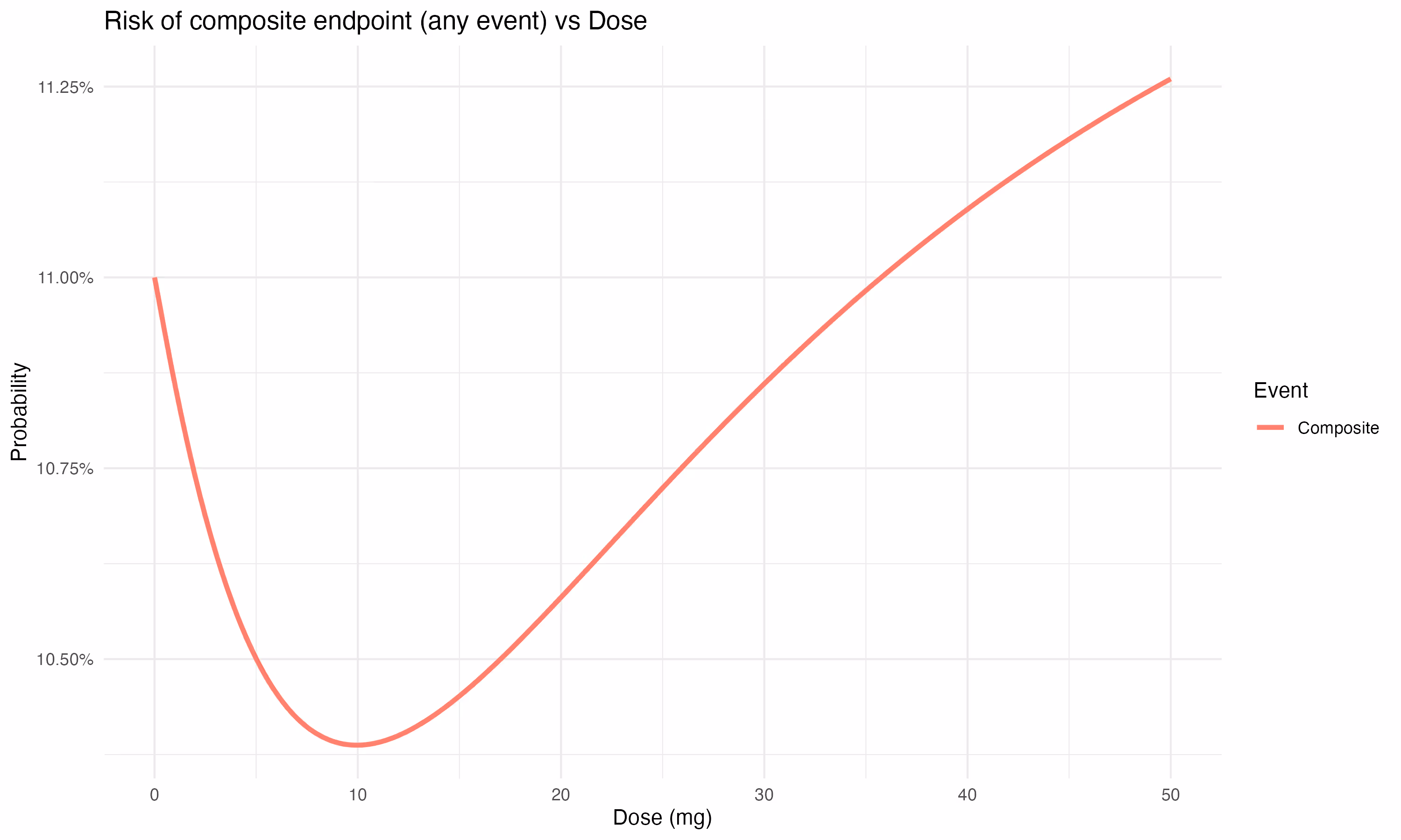
This is equivalent to using a standard approach of the composite endpoint (here: bleed or ischemic stroke).
However, different types of clinical events are rarely equal. Is the major bleed an intracranial hemorrhage (brain bleed)? Much worse than a major GI bleed.
This approach is overly simplistic for a number of reasons:
Finally, this decision is often made at a population level -- by which we mean that event rates are summarized over a population, and the optimal dose is selected (and given regulatory approval) for a population.
We see each of these complications as an opportunity for improvement.
How should we make an informed dosing decision?
Before we consider black-box methods like AI for improving medical decision-making, let's start embracing complexity and using the best tools available for analysis. Particularly those where the method is known and transparent. The learnings will transfer from these environments to the future we are hoping for.
Every dosing decision implies a particular utility that we are maximizing. A composite endpoint, for example, maximizes the avoidance of any of the composite’s events. But, we can elaborate on the utility function approach, to:
As an example of a degree-of-harmfulness score, we can consider the following ranking:
In practice, a patient or physician would set these according to their preference. For the example above, a higher weight on the bleed risk would result in a lower optimal dose, whereas a higher weight on stroke events would increase the optimal dose.
We [1] have developed a model with a goal of supporting rational decision making for dosing. This is a multi-state model estimated jointly with an exposure (pharmacokinetic) sub-model.
More details about this model are available in our poster [2].
At a minimum, our goals are to:
As we implemented this, we learned a few things. My goal in this post is to highlight them here.
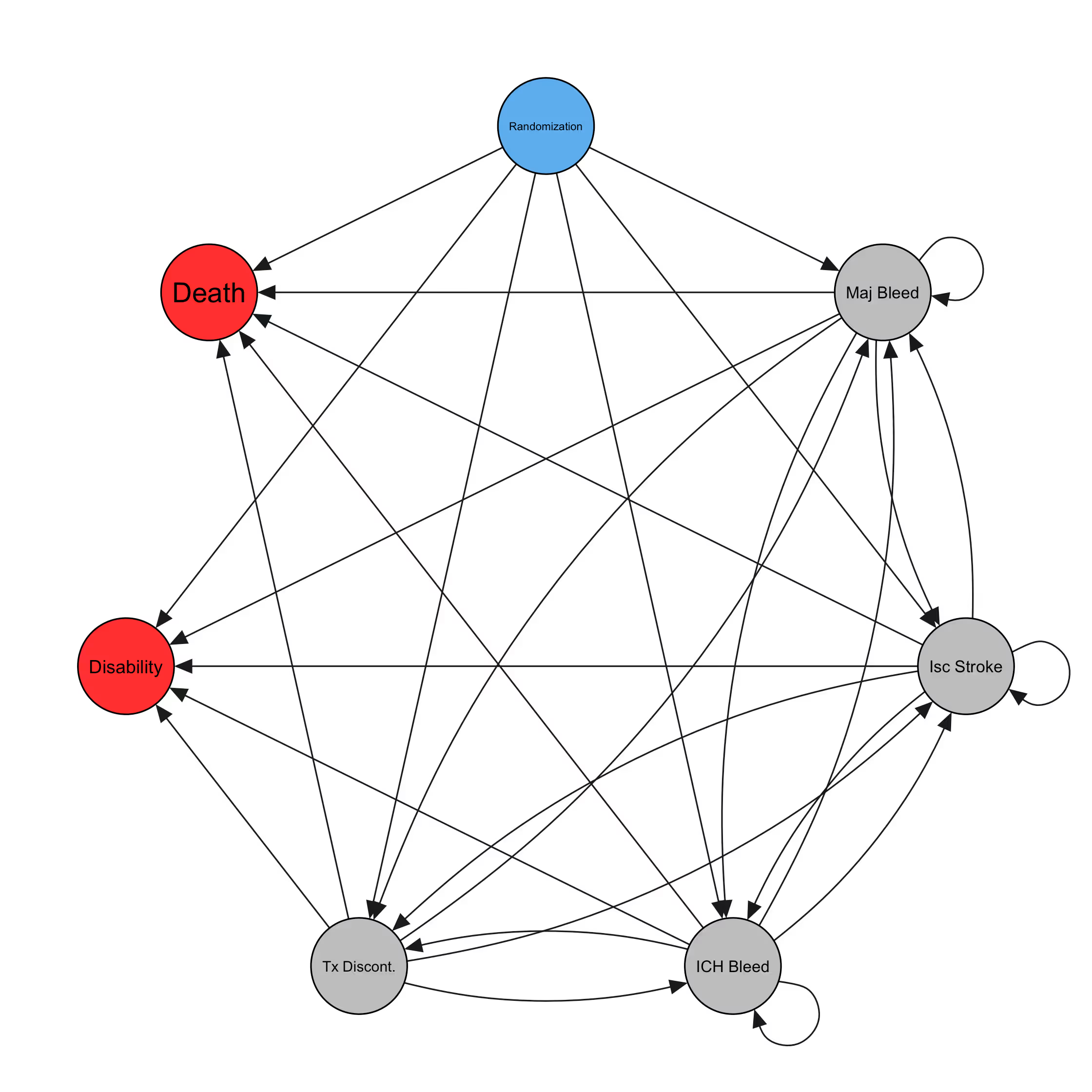
We start by considering the event graph. This defines which events are included in the model, and which possible transitions the model will consider.
For an anticoagulant drug, the event graph might look something like this:
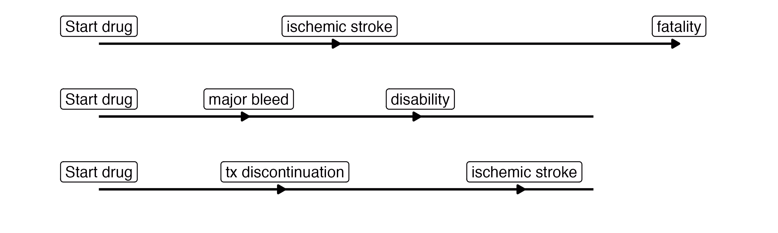
Many (perhaps most) subjects will have no events, and their paths are uneventful:

However, some patients will have more eventful journeys, such as
This graph is quite complicated. And yet, we are still leaving out several clinically-relevant events such as clinically-relevant non-major bleeds and minor bleeds, which likely increase the rate of treatment discontinuation. We are also missing cardiac events like myocardial infarctions and SEE. There is clearly a need for parsimony, here. This was our first learning. Our goal in building out the event graph is now to include events that influence the dosing decision. An event should either be explicitly part of the utility (e.g. death) or it should meaningfully inform the rate of events that are part of the utility. Because the number of possible transitions increases exponentially as we add events, we want to be judicious when selecting the ones to include.
A cool side-effect of this event graph is the inclusion of patient-oriented outcomes like fatality and long-term disability. These allow us to estimate the expected net effect of a change in dose on each, including any increased risk of fatality due to increased risk of stroke or ICH. This allows for a considerably simpler approach to the utility elicitation -- a dose decision can be made on the basis of reducing overall fatality and long-term disability, rather than asking the user to provide weights for each of 6 event types.
Also, this begs the question of why not take this to the extreme? We could theoretically simplify the graph further to focus on a single event at a time? The answer depends a bit on the specific dataset, but this is the topic of our JSM poster [2] and the manuscript in preparation.
Given the event graph, we then want to understand how treatment (dose) impacts the probability of each transition. A transition in this context is an event occurrence. We also include the influence of baseline covariates on each transition probability, since we have learned that the baseline risk of each event type (for a given patient) can dramatically impact the dosing decision.
The log likelihood is built up for each subject $i$, observed transition $k$ among those observed for this subject, and possible transition $h$ (each arrow in the graph above) as:
$$
\log p(\mathcal{D}_{\mathrm{MS}} \mid \theta) =
\sum_{i=1}^{N} \sum_{k=1}^{K_i} \sum_{h=1}^{H}
\left[
\delta_{k,i}^{(h)} \log\!\big(\lambda_i^{(h)}(t^{(i)}_k \mid \theta)\big)
- \mathrm{I}_{k,i}^{(h)} \int_{t^{(i)}_{k-1}}^{t^{(i)}_{k}}
\lambda_i^{(h)}(t \mid \theta) \, \mathrm{d}t
\right].
$$
Here, $\theta = \{\theta_0, \beta\}$ contains all model parameters, including the baseline hazard parameters $\theta_0$ and regression coefficients $\beta$.
For each transition $h = 1, \ldots, H$ and observation unit $n = 1, \ldots, N$, the hazard rates $\lambda^{(h)}_n(t \mid \theta)$, $h = 1, \ldots, H$, are modeled as
$$
\lambda^{(h)}_n(t \mid \theta) = b^{(h)}(t\mid \theta_0) \cdot \exp\left( \beta_{e_h}^{\top} \tilde{\mathbf{x}}_n \right)
$$
It's obvious in retrospect, but the covariates are surprisingly important not only for improving inference about the dose effects, but also for selecting the optimal dose for a patient. This seems like a large opportunity to improve dosing decisions by improving our ability to estimate baseline event risk for patients as they are being treated.
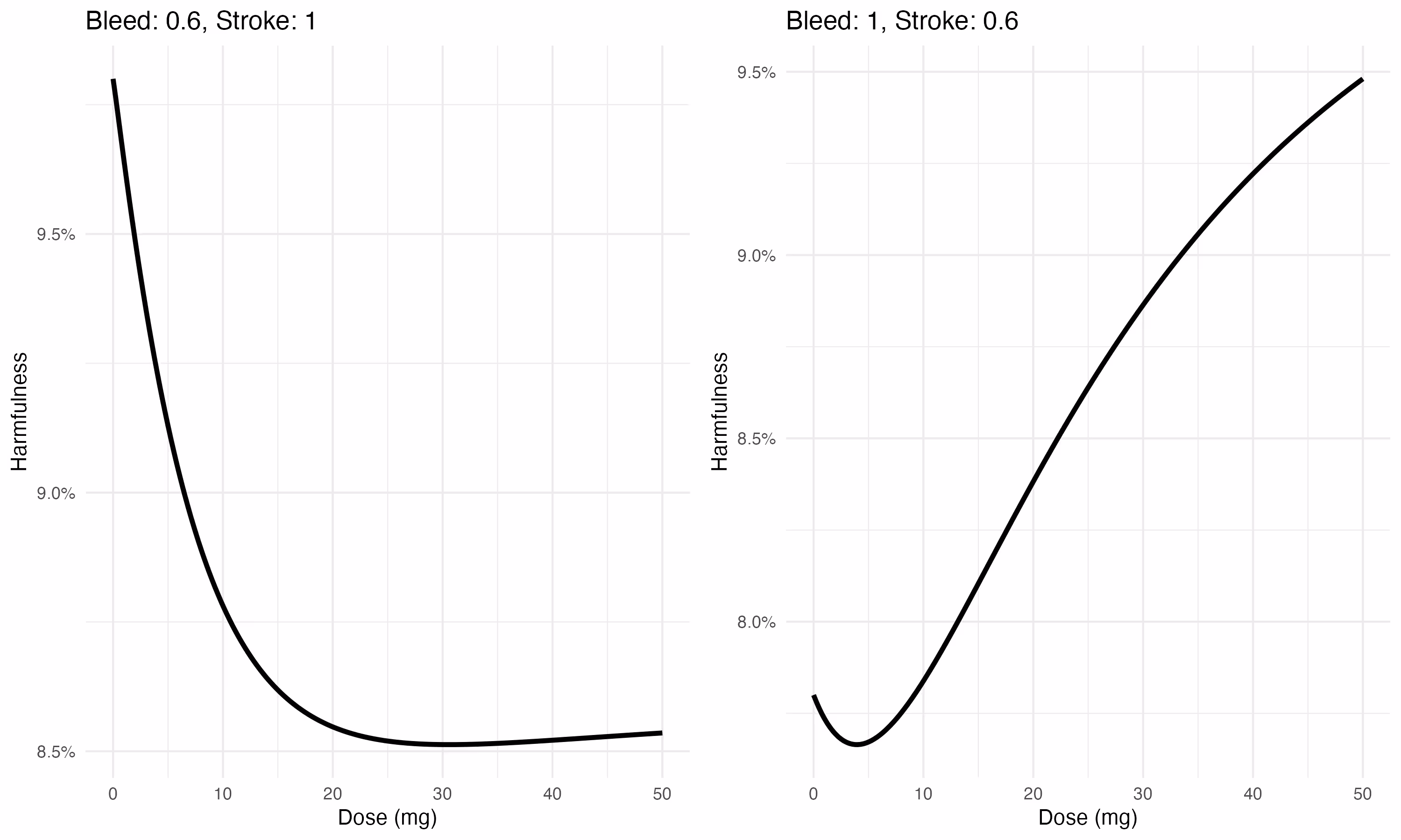
This is the next learning I want to share with you here. When considering more than one event, the optimal dose will depend on both the relative risk of events according to dose AND on the expected base rate of said events. This latter expectation is independent of dose.
To understand how this works, consider this version of the risks shown above, but this time for a patient with a particularly high stroke risk

Here, for a patient with high bleeding risk

These are from a simple shiny app - available on github if you want to play with it yourself.
Notice how the composite risk changes as we vary the baseline risk for each event, while holding the relative risk the same. Since so many dosing decisions are made at a population level, this suggests there is room to improve dosing by incorporating patient-level (covariate-adjusted) estimates of baseline event risk, rather than relying only on the population-level estimate.
[1] This is a joint work with TIMI Study Group, Cardiovascular Division, Brigham and Women’s Hospital, Department of Medicine, Harvard Medical School, Baim Institute for Clinical Research, and Daiichi Sankyo Inc.
[2] Timonen, J., Novik, E., Giugliano, R. P., Chen, C., Fronk, E.-M., Unverdorben, M., Clasen, M., Michael Gibson, C., & Buros, J. (2025). Personalized Dosing Decisions Using a Bayesian Exposure-Hazard Multistate Model. Joint Statistical Meetings, Nashville, TN. https://ww2.amstat.org/meetings/jsm/2025/
This is a comment related to the post above. It was submitted in a form, formatted by Make, and then approved by an admin. After getting approved, it was sent to Webflow and stored in a rich text field.
This is a comment related to the post above. It was submitted in a form, formatted by Make, and then approved by an admin. After getting approved, it was sent to Webflow and stored in a rich text field.
This is a comment related to the post above. It was submitted in a form, formatted by Make, and then approved by an admin. After getting approved, it was sent to Webflow and stored in a rich text field.
This is a comment related to the post above. It was submitted in a form, formatted by Make, and then approved by an admin. After getting approved, it was sent to Webflow and stored in a rich text field.
This is a comment related to the post above. It was submitted in a form, formatted by Make, and then approved by an admin. After getting approved, it was sent to Webflow and stored in a rich text field.
This is a comment related to the post above. It was submitted in a form, formatted by Make, and then approved by an admin. After getting approved, it was sent to Webflow and stored in a rich text field.
This is a comment related to the post above. It was submitted in a form, formatted by Make, and then approved by an admin. After getting approved, it was sent to Webflow and stored in a rich text field.
This is a comment related to the post above. It was submitted in a form, formatted by Make, and then approved by an admin. After getting approved, it was sent to Webflow and stored in a rich text field.
This is a comment related to the post above. It was submitted in a form, formatted by Make, and then approved by an admin. After getting approved, it was sent to Webflow and stored in a rich text field.
This is a comment related to the post above. It was submitted in a form, formatted by Make, and then approved by an admin. After getting approved, it was sent to Webflow and stored in a rich text field.
This is a comment related to the post above. It was submitted in a form, formatted by Make, and then approved by an admin. After getting approved, it was sent to Webflow and stored in a rich text field.
This is a comment related to the post above. It was submitted in a form, formatted by Make, and then approved by an admin. After getting approved, it was sent to Webflow and stored in a rich text field.
This is a comment related to the post above. It was submitted in a form, formatted by Make, and then approved by an admin. After getting approved, it was sent to Webflow and stored in a rich text field.
This is a comment related to the post above. It was submitted in a form, formatted by Make, and then approved by an admin. After getting approved, it was sent to Webflow and stored in a rich text field.
This is a comment related to the post above. It was submitted in a form, formatted by Make, and then approved by an admin. After getting approved, it was sent to Webflow and stored in a rich text field.
This is a comment related to the post above. It was submitted in a form, formatted by Make, and then approved by an admin. After getting approved, it was sent to Webflow and stored in a rich text field.
This is a comment related to the post above. It was submitted in a form, formatted by Make, and then approved by an admin. After getting approved, it was sent to Webflow and stored in a rich text field.
This is a comment related to the post above. It was submitted in a form, formatted by Make, and then approved by an admin. After getting approved, it was sent to Webflow and stored in a rich text field.
This is a comment related to the post above. It was submitted in a form, formatted by Make, and then approved by an admin. After getting approved, it was sent to Webflow and stored in a rich text field.
This is a comment related to the post above. It was submitted in a form, formatted by Make, and then approved by an admin. After getting approved, it was sent to Webflow and stored in a rich text field.
This is a comment related to the post above. It was submitted in a form, formatted by Make, and then approved by an admin. After getting approved, it was sent to Webflow and stored in a rich text field.
This is a comment related to the post above. It was submitted in a form, formatted by Make, and then approved by an admin. After getting approved, it was sent to Webflow and stored in a rich text field.
This is a comment related to the post above. It was submitted in a form, formatted by Make, and then approved by an admin. After getting approved, it was sent to Webflow and stored in a rich text field.
This is a comment related to the post above. It was submitted in a form, formatted by Make, and then approved by an admin. After getting approved, it was sent to Webflow and stored in a rich text field.
This is a comment related to the post above. It was submitted in a form, formatted by Make, and then approved by an admin. After getting approved, it was sent to Webflow and stored in a rich text field.
This is a comment related to the post above. It was submitted in a form, formatted by Make, and then approved by an admin. After getting approved, it was sent to Webflow and stored in a rich text field.
This is a comment related to the post above. It was submitted in a form, formatted by Make, and then approved by an admin. After getting approved, it was sent to Webflow and stored in a rich text field.

Trying to cut corners to make nonlinear PK model fitting faster

.svg)


This is a comment related to the post above. It was submitted in a form, formatted by Make, and then approved by an admin. After getting approved, it was sent to Webflow and stored in a rich text field.