

For a time-to-event model people usually just define a hazard function. What does it mean? If $T$ is the non-negative random variable representing the time when the event occurs for the first time, what does a given hazard function tell us about the distribution of $T$? How noisy will the data be if I generate data of $T$ with a given hazard function?
For comparing different time-to-event models, the concordance index (C-index) is a common choice. What is the expected C-index for an oracle model that knows the true hazard exactly?
The definition of a hazard function is
$$
h(t)
= \lim_{\Delta t \to 0}
\frac{P\big(t \le T < t + \Delta t \,\big|\, T \ge t\big)}{\Delta t}
$$
so a hazard function encodes the assumptions about the distribution of $T$. But
how does it relate to for example the probability density function $f_T(t)$
of $T$? Well, we see that
$$
\begin{align}
h(t)
&= \lim_{\Delta t \to 0}
\frac{P\big(t \le T < t + \Delta t\big)}{P(T\geq t) \Delta t} = \frac{1}{P(T\geq t)}\lim_{\Delta t \to 0}
\frac{P\big(t \le T < t + \Delta t\big)}{ \Delta t} = \frac{f_T(t)}{P(T\geq t)}
\end{align}
$$
where we used the rule of conditional probability and definition of a probability density. So the key identity is
$$
h(t) = \frac{\frac{\text{d}}{\text{d}t}F_T(t)}{1-F_T(t)}
$$
where $F_T(t) = P(T \leq t)$ is the cumulative distribution function (CDF) of $T$. Using
the survival function notation $S(t) = 1 - F_T(t) = P(T \geq t)$, we get
$$
h(t) = \frac{\frac{\text{d}}{\text{d}t}(1-S(t))}{S(t)} = \frac{- \frac{\text{d}}{\text{d}t} S(t)}{S(t)} = - \frac{\text{d}}{\text{d}t } \log S(t)
$$
which leads to
$$
S(t) = \exp \left(-\int_0^t h(u) \text{d}u \right).
$$
An additional feature of time-to-event data is censoring. We typically observe right-censored data, meaning that the event time $T$ is either observed at $t$, or we just observe that its value has to be larger than $t_{\text{max}}$.
This still isn't very concrete, so let us take an example. If we have a constant hazard $h(t) = h_0$, we get
$$
S(t) = \exp(-h_0 t)
$$
and
$$
F_T(t) = 1 - \exp(-h_0 t)
$$
which happens to be the CDF of the exponential distribution with rate $h_0$.
Now let us assume that we have subjects of different age, and the hazard is
$$
h(t) = h_x = \exp(\log \lambda_0 + \beta x)
$$
where $x$ is the normalized subject age. The below R functions can be used to simulate event data so that the original age is drawn uniformly from $[30, 90]$.
library(dplyr)
library(survival)

# True hazard rate
hazard <- function(log_h0, x, beta) {
  exp(log_h0 + beta * x)
}

# Simulate data
simulate_data <- function(N, log_h0, beta) {
  age <- stats::runif(N, min = 30, max = 90)
  norm_age <- (age - mean(age)) / sd(age)
  rate <- hazard(log_h0, norm_age, beta)
  t <- rexp(N, rate = rate)
  data.frame(subject = 1:N, event_time = t, age, norm_age)
}

# Censor event time
apply_censor <- function(df, tmax, log_h0, beta) {
  df$time <- pmin(df$event_time, tmax)
  df$status <- as.numeric(df$time != tmax)
  df$surv_time <- survival::Surv(df$time, df$status)
  df$surv_prob <- exp(-tmax * hazard(log_h0, df$norm_age, beta))
  df
}
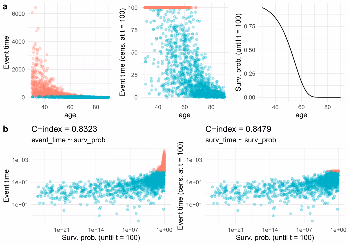
I use these to generate an event time for 2000 subjects so that $\beta=2$ and $\log \lambda_0 = -4$. On the upper row (a) of the below plot I visualize the distribution of event times over subjects, as well as the true probability of surviving until time $t_{\text{max}}=100$, which is $S(100) = \exp(-100 h_ x)$.
In survival analysis, the C-index of a prediction is computed as the proportion of concordant subject pairs divided by the total number of comparable subject pairs. A pair is concordant if the one with the earlier event time has a higher predicted risk (lower survival probability). A pair is comparable if we can unambiguously determine which subject had the earlier event (event times of both can't be censored). The maximum value is 1 (subjects ordered by survival probability are in the same order as the observed event times) and value 0.5 corresponds to random guessing.
On the bottom row (b) of the previous plot is the event time as a function of the true survival probability. Also, I have computed the C-index which tells how concordant the predictions (survival probabilities until $t=100$) are with the fully observed event times (event_time) or the censored versions (surv_time). Now, this is the oracle model which knows the true event probability, but it doesn't achieve a perfect C-index of 1. This is because the event time data is "noisy", meaning that a subject A who has a higher hazard than subject B, can get a lower event time realization than subject B. So what is the theoretical maximum that we can achieve, and how does it depend on the different factors $\lambda_0$, $t_{\text{max}}$ and $\beta$?
The below R function can be used to simulate data and compute the concordance index with a given number of subjects $N$, value of $\log(\lambda_0)$, $t_ {\text{max}}$ and $\beta$.
library(dplyr)
library(survival)
compute_ci <- function(N, log_base_rate, tmax, beta) {
  df <- simulate_data(N, log_base_rate, beta)
  df_cens <- apply_censor(df, tmax, log_base_rate, beta)
  ci1 <- survival::concordance(event_time ~ surv_prob, data = df_cens)
  ci2 <- survival::concordance(surv_time ~ surv_prob, data = df_cens)
  data.frame(
    N = N, log_base_rate = log_base_rate, tmax = tmax,
    beta = beta,
    Noncensored = as.numeric(ci1$concordance),
    Censored = as.numeric(ci2$concordance)
  )
}
Note that in this case I could just use formulas like event_time ~ age because the ordering by age is same as the ordering by survival probability. In fact, I could use anything that is a strictly monotonic function of age and get the same C-index.
Now, how does the C-index of the oracle depend on $t_ {\text{max}}$, $\log(\lambda_0)$ and $\beta$? This question is answered by the panels a, b, and c of the below plot. Below, we go through what we see in the panels one by one.
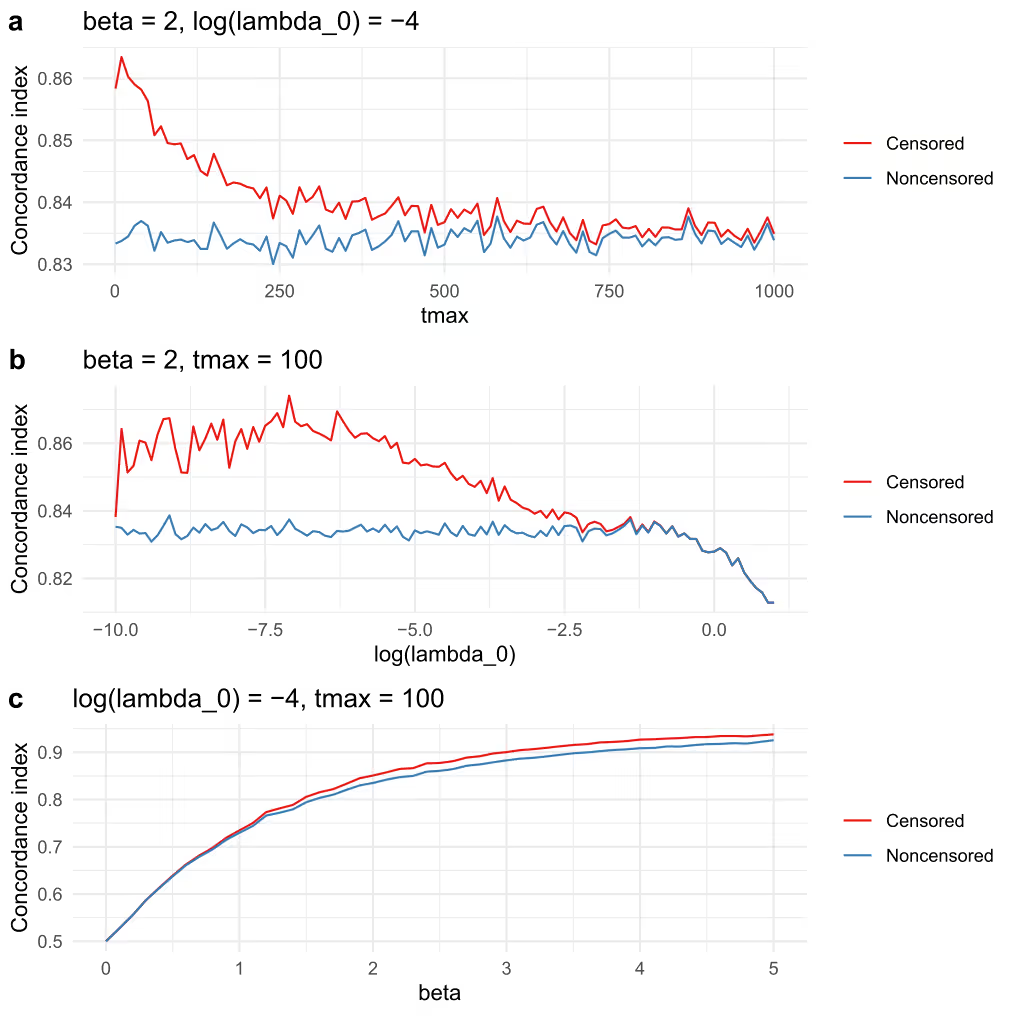
Something that was not yet discussed is how to handle ties for C-index, because with a unique age for each subject and $\beta>0$, there cannot be ties in the survival probability. This would change and affect the results if we rounded age to for example years, in which case the subjects with the same age have the same predicted survival probability. Also, in the special case $\beta=0$ all subjects have the same predicted survival probability. We see in panel c), that in this case the C-index is 0.5, because a tied pair is counted as half-concordant by the underlying implementation (Harrel's C).
More ties will occur if instead of the one-year resolution we discretize the data in to a few age groups. The number of possible unique survival probability predictions is same as the number of unique groups. Now, assume the Harrel's C definition of C-index and no censoring (all subject pairs are comparable), just two groups, and equal group sizes. Let $h_1$ and $h_2 > h_1$ be the hazards of group 1 and 2, respectively. A key insight is that if we draw values $T_1$ and $T_2$ from the exponential distribution with rates $h_1$ and $h_2$, respectively, then
$$P(T_2 < T_1) = \frac{h_2}{h_1 + h_2}.$$
However, the C-index definition is
$$
C = \frac{1 \times \text{number of concordant subject pairs} + 0.5 \times \text{number of tied subject pairs}}{\text{total number of subject pairs}}
$$ so if we generate data, the expected value is
$$E[C] = P(\text{random pair is tied}) \times 0.5 + P(\text{random pair is not tied and is concordant}) \times 1.$$ A random pair of subjects are from the same group with probability 0.5, so $ P(\text{random pair is tied})=0.5$. The expected value of the C-index of the oracle model is therefore
$$E[C] = 0.5 \cdot 0.5 + 0.5 \frac{h_2}{h_1 + h_2} = 0.25 + 0.5 \frac{\frac{h_2}{h_1}}{1 + \frac{h_2}{h_1}}.$$
Now, even if the hazard ratio $ \frac{h_2}{h_1} \rightarrow \infty$, we have $E[C] \rightarrow 0.75 < 1$.
When thinking about whether the C-index of your model is good, it helps to think what the C-index of the true data-generating hazard model could ideally be if you generated similar data from it. The larger the difference in true hazards between the subjects is, the higher the achievable C-index.
This is a comment related to the post above. It was submitted in a form, formatted by Make, and then approved by an admin. After getting approved, it was sent to Webflow and stored in a rich text field.
This is a comment related to the post above. It was submitted in a form, formatted by Make, and then approved by an admin. After getting approved, it was sent to Webflow and stored in a rich text field.
This is a comment related to the post above. It was submitted in a form, formatted by Make, and then approved by an admin. After getting approved, it was sent to Webflow and stored in a rich text field.
This is a comment related to the post above. It was submitted in a form, formatted by Make, and then approved by an admin. After getting approved, it was sent to Webflow and stored in a rich text field.
This is a comment related to the post above. It was submitted in a form, formatted by Make, and then approved by an admin. After getting approved, it was sent to Webflow and stored in a rich text field.
This is a comment related to the post above. It was submitted in a form, formatted by Make, and then approved by an admin. After getting approved, it was sent to Webflow and stored in a rich text field.
This is a comment related to the post above. It was submitted in a form, formatted by Make, and then approved by an admin. After getting approved, it was sent to Webflow and stored in a rich text field.
This is a comment related to the post above. It was submitted in a form, formatted by Make, and then approved by an admin. After getting approved, it was sent to Webflow and stored in a rich text field.
This is a comment related to the post above. It was submitted in a form, formatted by Make, and then approved by an admin. After getting approved, it was sent to Webflow and stored in a rich text field.
This is a comment related to the post above. It was submitted in a form, formatted by Make, and then approved by an admin. After getting approved, it was sent to Webflow and stored in a rich text field.
This is a comment related to the post above. It was submitted in a form, formatted by Make, and then approved by an admin. After getting approved, it was sent to Webflow and stored in a rich text field.
This is a comment related to the post above. It was submitted in a form, formatted by Make, and then approved by an admin. After getting approved, it was sent to Webflow and stored in a rich text field.
This is a comment related to the post above. It was submitted in a form, formatted by Make, and then approved by an admin. After getting approved, it was sent to Webflow and stored in a rich text field.
This is a comment related to the post above. It was submitted in a form, formatted by Make, and then approved by an admin. After getting approved, it was sent to Webflow and stored in a rich text field.
This is a comment related to the post above. It was submitted in a form, formatted by Make, and then approved by an admin. After getting approved, it was sent to Webflow and stored in a rich text field.
This is a comment related to the post above. It was submitted in a form, formatted by Make, and then approved by an admin. After getting approved, it was sent to Webflow and stored in a rich text field.
This is a comment related to the post above. It was submitted in a form, formatted by Make, and then approved by an admin. After getting approved, it was sent to Webflow and stored in a rich text field.
This is a comment related to the post above. It was submitted in a form, formatted by Make, and then approved by an admin. After getting approved, it was sent to Webflow and stored in a rich text field.
This is a comment related to the post above. It was submitted in a form, formatted by Make, and then approved by an admin. After getting approved, it was sent to Webflow and stored in a rich text field.
This is a comment related to the post above. It was submitted in a form, formatted by Make, and then approved by an admin. After getting approved, it was sent to Webflow and stored in a rich text field.
This is a comment related to the post above. It was submitted in a form, formatted by Make, and then approved by an admin. After getting approved, it was sent to Webflow and stored in a rich text field.
This is a comment related to the post above. It was submitted in a form, formatted by Make, and then approved by an admin. After getting approved, it was sent to Webflow and stored in a rich text field.
This is a comment related to the post above. It was submitted in a form, formatted by Make, and then approved by an admin. After getting approved, it was sent to Webflow and stored in a rich text field.
This is a comment related to the post above. It was submitted in a form, formatted by Make, and then approved by an admin. After getting approved, it was sent to Webflow and stored in a rich text field.
This is a comment related to the post above. It was submitted in a form, formatted by Make, and then approved by an admin. After getting approved, it was sent to Webflow and stored in a rich text field.
This is a comment related to the post above. It was submitted in a form, formatted by Make, and then approved by an admin. After getting approved, it was sent to Webflow and stored in a rich text field.
This is a comment related to the post above. It was submitted in a form, formatted by Make, and then approved by an admin. After getting approved, it was sent to Webflow and stored in a rich text field.

Trying to cut corners to make nonlinear PK model fitting faster
.svg)


This is a comment related to the post above. It was submitted in a form, formatted by Make, and then approved by an admin. After getting approved, it was sent to Webflow and stored in a rich text field.