Chaos and numerics

Predicting chaos

Differential equation systems such as the double pendulum, the three-body problem, and the Lorenz system can be chaotic. This means that a slight perturbation in the initial condition leads to a (qualitatively) very different future state of the system. This is a problem because it means that if we cannot measure the current state (position of planets, angles of pendulum, weather) exactly, there is no point in trying to predict the long-term future (even if the system would somehow exactly capture the laws of nature).

In this post I have a slightly different angle. Let's say that we do know the initial state exactly. There is still the problem of representing that state numerically on the computer, and errors that accumulate when predicting the future. Therefore this post can be seen as continuation to my earlier post. The running example is the Lorenz system

$$
\begin{align}
\dot{x} &= \sigma (y - x), \\
\dot{y} &= x(\rho - z) - y, \\
\dot{z} &= xy - \beta z.
\end{align}
$$

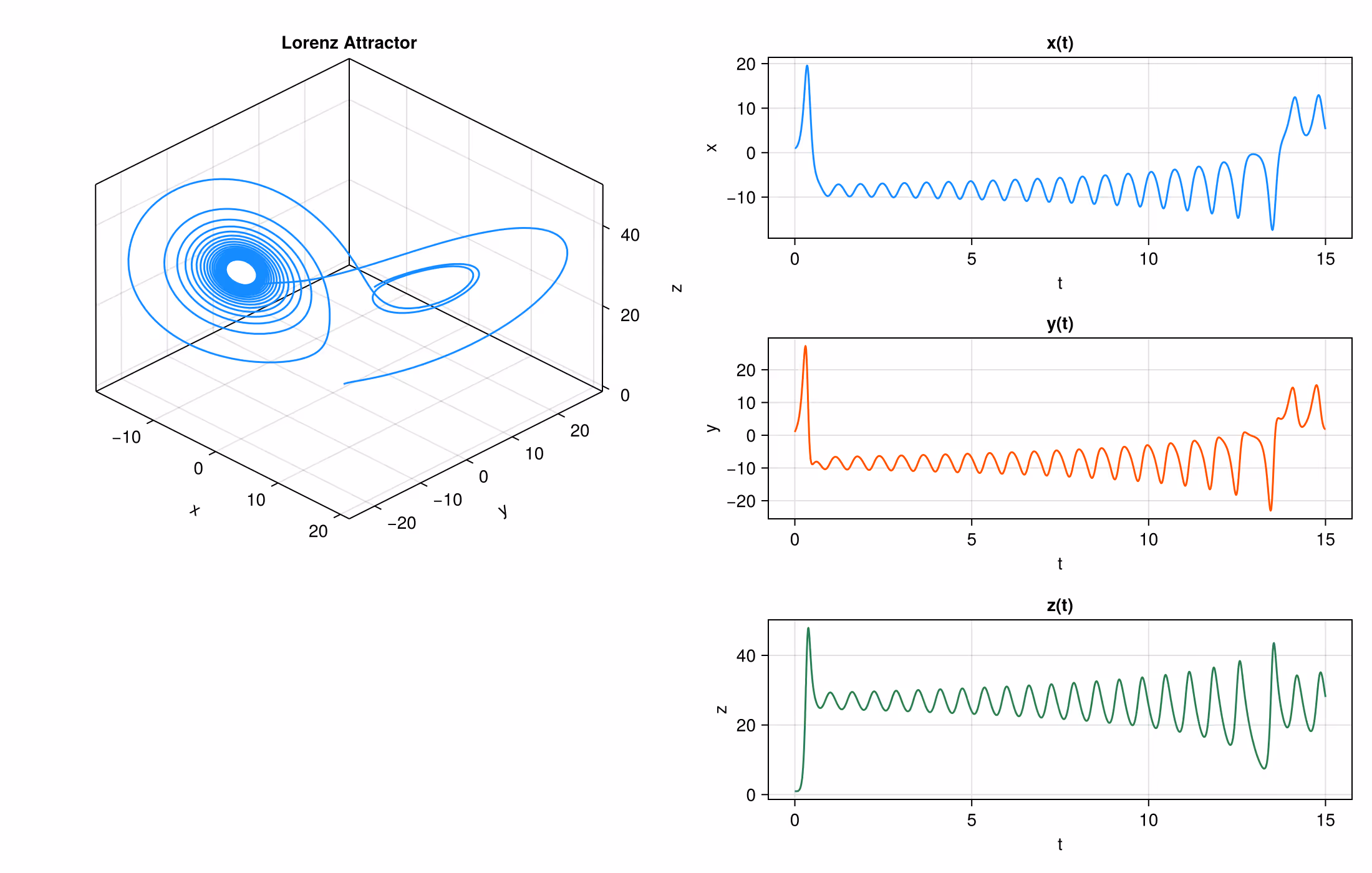
with parameter values $\sigma=10$, $\rho=28$, $\beta=\frac{8}{3}$. With these values, it is called the Lorenz attractor, because almost all initial conditions lead to similar looking butterfly-shaped trajectories.

‍

Dependency on the numerical solver

We must use a numerical ODE solver to study the behaviour of the system. Here is Julia code for simulating it.
‍

# Lorenz system derivative
function lorenz!(du, u, p, t)
    σ, ρ, β = p
    du[1] = σ * (u[2] - u[1])
    du[2] = u[1] * (ρ - u[3]) - u[2]
    du[3] = u[1] * u[2] - β * u[3]
end

# Integrate the Lorenz system and return the solution object
function simulate_lorenz(; u0 = [1.0, 1.0, 1.0],
                            p = (10.0, 28.0, 8 / 3),
                            tspan = (0.0, 31.0),
                            dt = 0.01,
                            reltol = 1e-6,
                            abstol = 1e-6)
    prob = ODEProblem(lorenz!, u0, tspan, p)
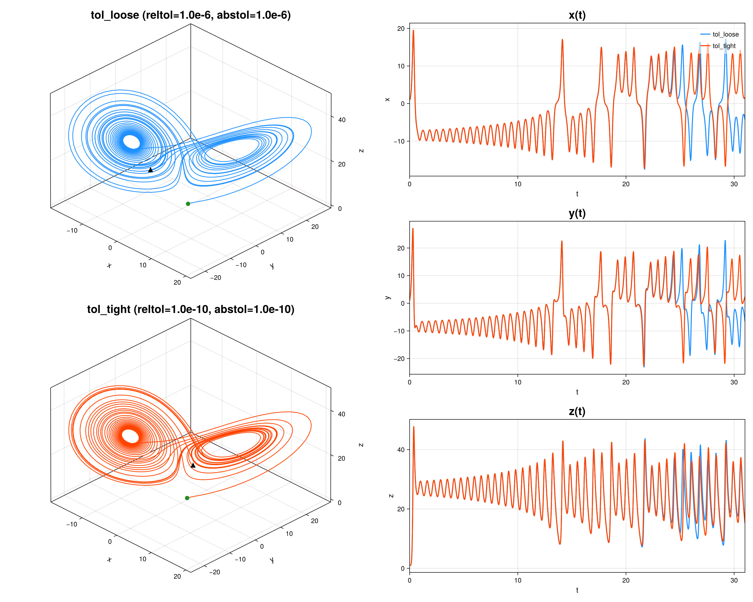
    solve(prob, Tsit5(); dt = dt, reltol = reltol, abstol = abstol)
end

We see that the Tsit5 solver is used. Below, I have plotted the solution in the state space and each component separately. I am comparing two different solver tolerance configurations. The blue line is using tolerances of $1e^{-6}$ and the red line is obtained with $1e^{-10}$. We see that the solutions agree well up until about $t=22$, after which they start to slightly differ, after which they quickly take qualitatively different trajectories. The end point ($t=31$), shown with the black triangle, is in the "left wing" of the butterfly in one solution, and in the "right wing" in the other.

‍

‍

‍

Dependency on floating point precision

In the above code, all computations happened in 64-bit float. We can define a templated version

# Lorenz system derivative (out-of-place, returns an SVector)
@inline function lorenz(u, p, t)
    σ, ρ, β = p
    SVector(σ * (u[2] - u[1]),
            u[1] * (ρ - u[3]) - u[2],
            u[1] * u[2] - β * u[3])
end

# Integrate the Lorenz system with a chosen floating-point type
function simulate_lorenz(::Type{T};
                         u0 = (1, 1, 1),
                         p = (10, 28, 8 / 3),
                         tspan = (0, 31),
                         dt = 0.01,
                         reltol = 1e-10,
                         abstol = 1e-10) where {T}
    u0T = SVector{3,T}(T.(u0))
    pT  = SVector{3,T}(T.(p))
    tspanT = (T(tspan[1]), T(tspan[2]))
    dtT = T(dt)
    prob = ODEProblem(lorenz, u0T, tspanT, pT)
    solve(prob, Tsit5(); dt = dtT, reltol = reltol, abstol = abstol)
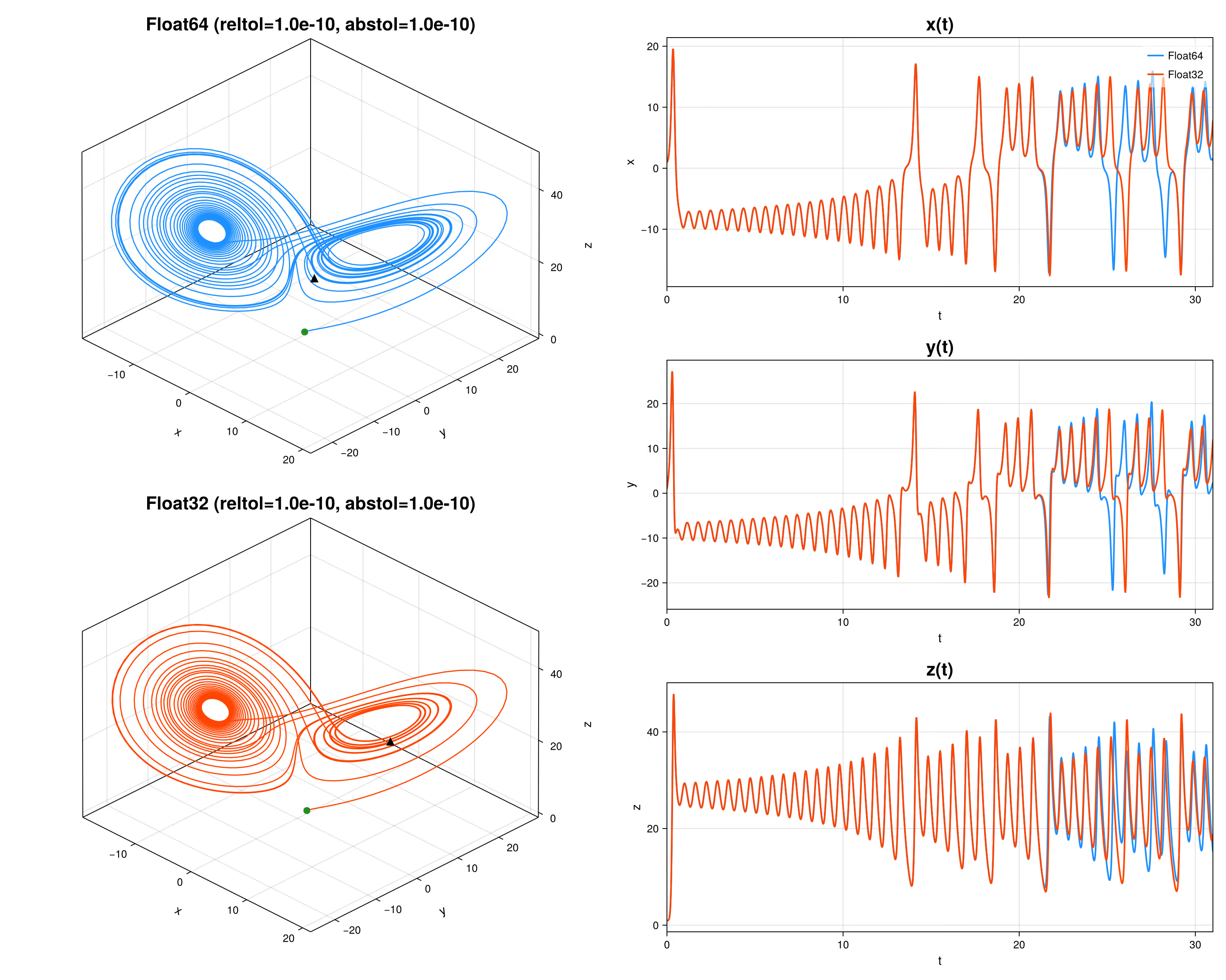
end

to study the effect of floating point precision. In the below plot I compare solutions with 64-bit and 32-bit floats. We see that again, they qualitatively start to differ when predicting far enough.

‍

‍

Lyapunov exponents

The maximal Lyapunov exponent is a way of quantifying the predictability of a system. It is a value $\lambda_{\max}$ such that, for infinitesimal initial separations $\textbf{d}_0$ and asymptotically in time,
$$
\lVert \textbf{d}(t) \rVert \sim e^{\lambda_{\max}t} \lVert \textbf{d}_0 \rVert
$$

where $\textbf{d}(t)$ is the difference of solutions at time $t$. In reality, even if we theoretically know the initial value (implying $\textbf{d}_0= \textbf{0}$), there will still be the floating point error, so $\lVert \textbf{d}_0 \rVert > 0$. And since the Lorenz attractor has a positive $\lambda_{\max} \approx 0.9$, long-term prediction is difficult.

Luckily we typically work with much simpler systems. Consider a one-compartment pharmacokinetic model with first-order oral absorption and linear elimination, defined as
$$
\begin{align}
\dot A_g &= -k_a A_g, \\
\dot A_c &= k_a A_g - k_e A_c,
\end{align}
$$
where \(A_g\) and \(A_c\) denote the amounts in the gut and central compartment, and $k_a,k_e>0$. Defining the state vector
$$
\mathbf A =
\begin{bmatrix}
A_g \\ A_c
\end{bmatrix},
$$
the system can be written in matrix form as
$$
\dot{\mathbf A} = M \mathbf A,
\qquad
M =
\begin{bmatrix}
-k_a & 0 \\
k_a & -k_e
\end{bmatrix}.
$$For a linear time-invariant system such as this, Lyapunov exponents are given by the real parts of the eigenvalues of $M$. These satisfy
$$
\det(M-\lambda I)
=
(-k_a-\lambda)(-k_e-\lambda)=0,
$$
yielding
$$
\lambda_1=-k_a,
\qquad
\lambda_2=-k_e.
$$
Hence the Lyapunov spectrum is $\{-k_a,-k_e\}$, and the maximal Lyapunov exponent is
$$
\lambda_{\max}=\max(-k_a,-k_e)=-\min(k_a,k_e)<0,
$$
implying exponential decay of perturbations and global stability of the system.

‍

Parameter estimation and bifurcations

So far we assumed that the parameters that define the system are known, and only focused on the behaviour as a function of the initial condition and numerical inaccuracy. The study of how the qualitative behavior of dynamical systems changes as parameters vary is known as bifurcation theory. Existence of bifurcations and chaos will make parameter estimation very complicated, since even if your parameters are almost right, after a while the simulated trajectory won’t line up with observations at all. Parameter estimation across bifurcations and chaos might be possible, but probably requires abandoning the usual full trajectory matching to observations. Possible strategies include

• Fitting to short time windows
• Classifying/filtering out parameter regimes based on qualitative behaviour than can be derived using bifurcation theory
• Instead of observation model for the state variables, fit to invariant statistics or other properties (mean, variance, max value)
• Something else I don't know about

‍

‍

‍