

Last week, Juho wrote about our general approach to probabilistic inference, which focused on the flexible modeling of each subject's (could be a person, animal, or in-vitro sample) biomarker's response function, which can be written slightly more generally.
$$ y(x) \sim f(\mu(x \mid \theta), \sigma^2) $$
In a context of a clinical trial or multiple trials or real-world data (RWD) like electronic health records, multiple biomarker trajectories could be observed within a subject, and each subject is a member of a larger population such as trial, dose group, hospital, geographic region, etc. We can also observe multiple biomarker types.
When we model data, it is a good idea to respect this generative story and not prematurely collapse all observations as if they came from the same source, or compute per-source averages and feed those into the model — both result in loss of information, and in healthcare, information is expensive and hard to get.
Once we have a generative model for a dynamical process, like tumor growth or drug exposure, and the structure of where each measurement was taken, we can start putting it together into one model. This takes some work, but if successful, the benefits are usually worth it — in particular, we can make predictions at each level of the model — for each biomarker, individual, dose, trial-arm, and so on. In other words, we can do both individual and average treatment effect type of inference.
What would a model like this look like? The usual term is a hierarchical or multi-level model. In 2019, we worked with Sam Brilleman on a paper called "Joint longitudinal and time-to-event models for multilevel hierarchical data" [1], which describes one such model, with a caveat that the above function $f$ must come from an exponential family and form a GLM. Later, we have evolved these models to include a much more flexible choice of $f$.
Part of the paper was based on the analysis of AstraZeneca's IPASS trial. The IPASS trial (IRESSA Pan-Asia Study) was a pivotal Phase III, randomized, open-label clinical study investigating first-line treatment for advanced non-small cell lung cancer (NSCLC). The trial compared gefitinib (an EGFR tyrosine kinase inhibitor) to standard carboplatin/paclitaxel chemotherapy in clinically selected East Asian patients with advanced lung adenocarcinoma, explicitly focusing on never-smokers or former light smokers.
The core idea was to assess how the dynamics of tumor growth within each patient affect overall survival. This could be important for go/no-go decisions in Phase II, for example. Typically, the target lesion size is tracked over time, and the measurement unit is the sum of the longest diameter of all target lesions, as seen on a radiographic scan. In this case, we had access to each lesion, and the following figure shows this three-level hierarchical data structure in Panel (b).
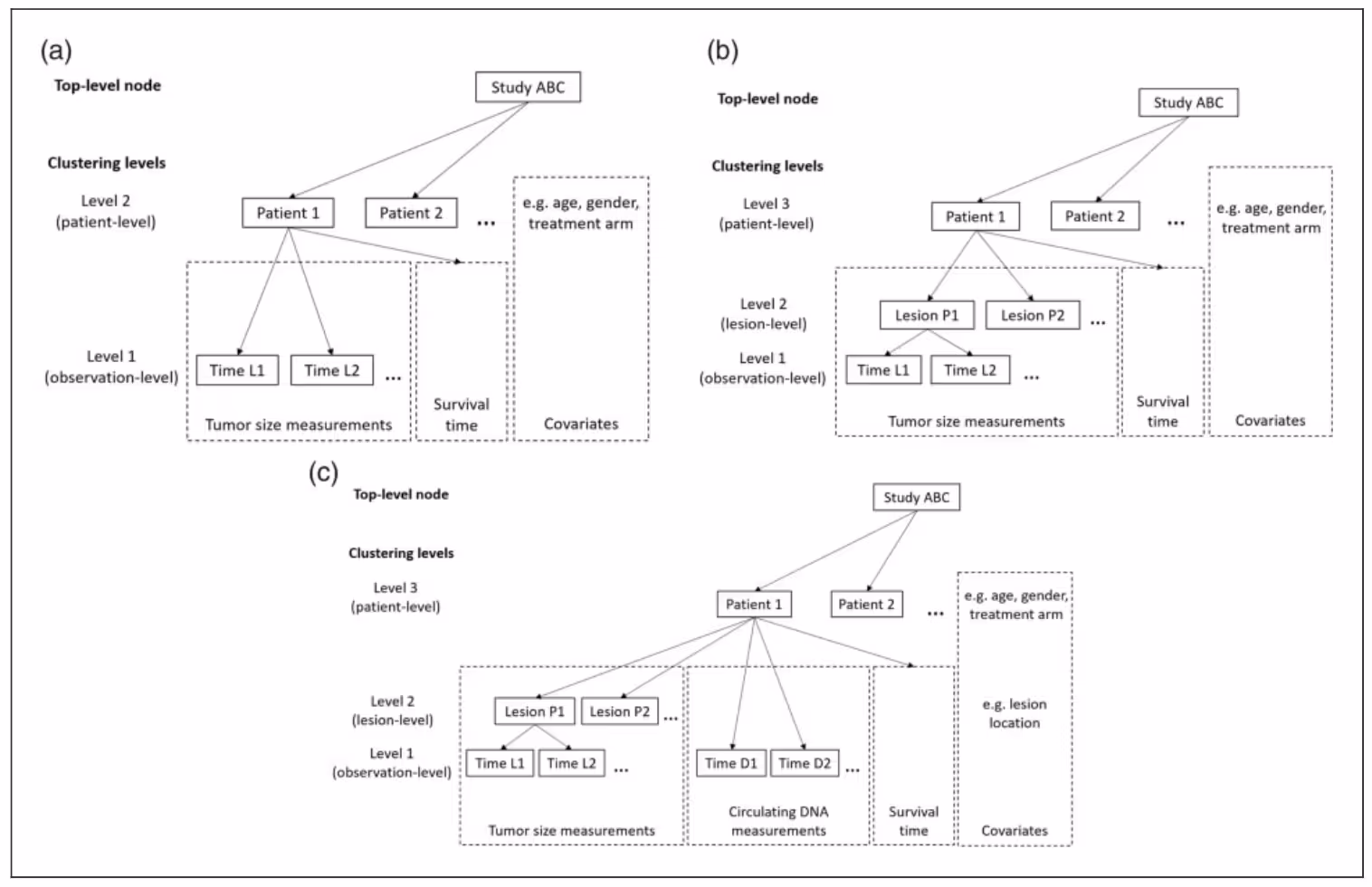
This framework enables us to support multiple biomarker types, not just multiple trajectories of the same biomarker, such as lesion size measurements over time. For example, in Panel (c), in addition to the lesion trajectories, we can track ctDNA measurements over time. In principle, there is no limit on the number of biomarker types; however, in practice, the computation becomes intractable once the number of marker types exceeds single digits.
Now, back to our three-level hierarchy. In a GLM setting, our this hierarchy can be encoded using the usual linear predictor $\eta$ and the conditional mean $\mu$ that is derived by transforming $\eta$ with a link function $g$, which for linear models would be identity.
$$ \begin{aligned}
\eta_{ij}(t) &= x_{ij}^\top(t)\,\beta + z_{ij}^\top(t)\,b_i + w_{ij}^\top(t)\,u_{ij} \\
\mu_{ij}(t) &= g^{-1}(\eta_{ij}(t))
\end{aligned} $$
The conditional mean function $\mu$ goes into the distributional function $f$ above to account for measurement noise. Patients are indexed by $i$ and lesions by $j$. Covariates can come in at every level and are represented by $x$, $z$, and $w$, with the corresponding study-level effects $\beta$ (sometimes called fixed effects), patient-level offsets $b_i$, and lesion-level offsets $u_{ij}$.
A more interesting bit is inside the event submodel, which is formulated using a traditional proportional hazards structure.
$$ h_i(t) = h_0(t; \boldsymbol{\omega}) \mathsf{exp} \left( \boldsymbol{w}^T_i(t) \boldsymbol{\gamma} + \sum_{m=1}^M \sum_{q=1}^{Q_m} f_{mq}(\boldsymbol{\beta}, \boldsymbol{b}_{i}, \alpha_{mq}; t) \right) $$
The most salient part is inside the $\exp$ and specifically under the summation over $M$ and $Q$. $Q$ in our case indexes lesion trajectories and if we had another marker like ctDNA, we would have $M = 2$.
The function $f_{qm}$, which is not the same as the $f$ defined at the beginning, can be any function that computes an informative aspect of the biomarker trajectory. Popular choices include the current value of the biomarker and the rate of change. In principle, the choices are infinite, and many have been implemented in rstanarm.
The coefficient $\alpha_{mq}$ is called the association parameter and is often the key estimand as it captures the strength of association between the biomarker model and the expected event rate.
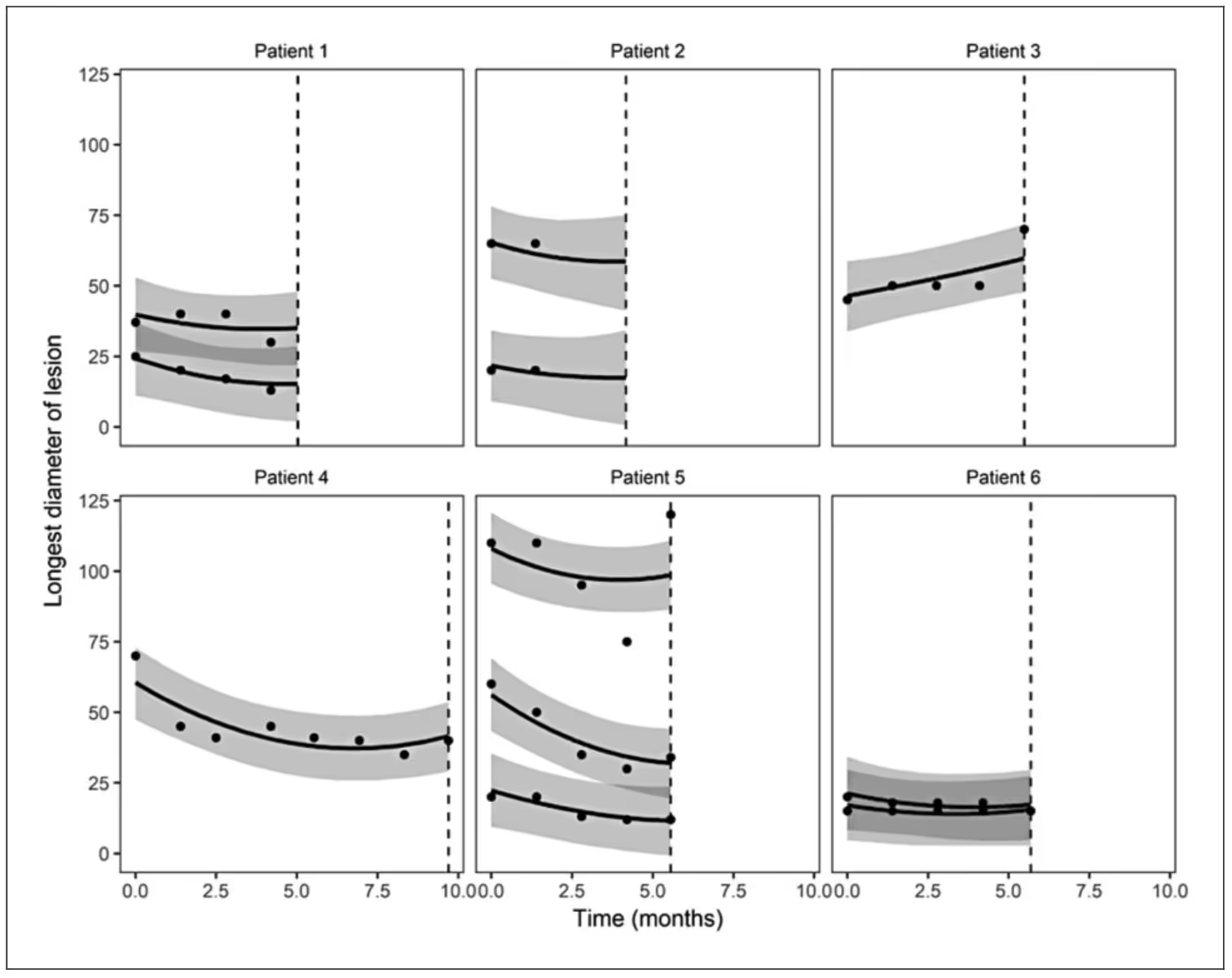
When Sam fit the model to the IPASS data, he used a linear model for lesions that was quadratic in time (i.e., identity link and normal distribution) and several association functions, including lesion-specific expected value and slope.
The following figure shows a small sample of patient-level prediction intervals with several patients having multiple lesions.
If you are interested in experimenting with these types of models, and assuming you are okay with the longitudinal submodel being a GLM, we have developed an open-source function inside the rstanarm package called stan_jm().
[1] Brilleman, S. L., Crowther, M. J., Moreno-Betancur, M., Buros Novik, J., Dunyak, J., Al-Huniti, N., Fox, R., Hammerbacher, J., & Wolfe, R. (2019). Joint longitudinal and time-to-event models for multilevel hierarchical data. Statistical Methods in Medical Research, 28(12), 3502–3515.
Preprint: https://arxiv.org/pdf/1805.06099
This is a comment related to the post above. It was submitted in a form, formatted by Make, and then approved by an admin. After getting approved, it was sent to Webflow and stored in a rich text field.
This is a comment related to the post above. It was submitted in a form, formatted by Make, and then approved by an admin. After getting approved, it was sent to Webflow and stored in a rich text field.
This is a comment related to the post above. It was submitted in a form, formatted by Make, and then approved by an admin. After getting approved, it was sent to Webflow and stored in a rich text field.
This is a comment related to the post above. It was submitted in a form, formatted by Make, and then approved by an admin. After getting approved, it was sent to Webflow and stored in a rich text field.
This is a comment related to the post above. It was submitted in a form, formatted by Make, and then approved by an admin. After getting approved, it was sent to Webflow and stored in a rich text field.
This is a comment related to the post above. It was submitted in a form, formatted by Make, and then approved by an admin. After getting approved, it was sent to Webflow and stored in a rich text field.
This is a comment related to the post above. It was submitted in a form, formatted by Make, and then approved by an admin. After getting approved, it was sent to Webflow and stored in a rich text field.
This is a comment related to the post above. It was submitted in a form, formatted by Make, and then approved by an admin. After getting approved, it was sent to Webflow and stored in a rich text field.
This is a comment related to the post above. It was submitted in a form, formatted by Make, and then approved by an admin. After getting approved, it was sent to Webflow and stored in a rich text field.
This is a comment related to the post above. It was submitted in a form, formatted by Make, and then approved by an admin. After getting approved, it was sent to Webflow and stored in a rich text field.
This is a comment related to the post above. It was submitted in a form, formatted by Make, and then approved by an admin. After getting approved, it was sent to Webflow and stored in a rich text field.
This is a comment related to the post above. It was submitted in a form, formatted by Make, and then approved by an admin. After getting approved, it was sent to Webflow and stored in a rich text field.
This is a comment related to the post above. It was submitted in a form, formatted by Make, and then approved by an admin. After getting approved, it was sent to Webflow and stored in a rich text field.
This is a comment related to the post above. It was submitted in a form, formatted by Make, and then approved by an admin. After getting approved, it was sent to Webflow and stored in a rich text field.
This is a comment related to the post above. It was submitted in a form, formatted by Make, and then approved by an admin. After getting approved, it was sent to Webflow and stored in a rich text field.
This is a comment related to the post above. It was submitted in a form, formatted by Make, and then approved by an admin. After getting approved, it was sent to Webflow and stored in a rich text field.
This is a comment related to the post above. It was submitted in a form, formatted by Make, and then approved by an admin. After getting approved, it was sent to Webflow and stored in a rich text field.
This is a comment related to the post above. It was submitted in a form, formatted by Make, and then approved by an admin. After getting approved, it was sent to Webflow and stored in a rich text field.
This is a comment related to the post above. It was submitted in a form, formatted by Make, and then approved by an admin. After getting approved, it was sent to Webflow and stored in a rich text field.
This is a comment related to the post above. It was submitted in a form, formatted by Make, and then approved by an admin. After getting approved, it was sent to Webflow and stored in a rich text field.
This is a comment related to the post above. It was submitted in a form, formatted by Make, and then approved by an admin. After getting approved, it was sent to Webflow and stored in a rich text field.
This is a comment related to the post above. It was submitted in a form, formatted by Make, and then approved by an admin. After getting approved, it was sent to Webflow and stored in a rich text field.
This is a comment related to the post above. It was submitted in a form, formatted by Make, and then approved by an admin. After getting approved, it was sent to Webflow and stored in a rich text field.
This is a comment related to the post above. It was submitted in a form, formatted by Make, and then approved by an admin. After getting approved, it was sent to Webflow and stored in a rich text field.
This is a comment related to the post above. It was submitted in a form, formatted by Make, and then approved by an admin. After getting approved, it was sent to Webflow and stored in a rich text field.
This is a comment related to the post above. It was submitted in a form, formatted by Make, and then approved by an admin. After getting approved, it was sent to Webflow and stored in a rich text field.
This is a comment related to the post above. It was submitted in a form, formatted by Make, and then approved by an admin. After getting approved, it was sent to Webflow and stored in a rich text field.

Trying to cut corners to make nonlinear PK model fitting faster

.svg)

This is a comment related to the post above. It was submitted in a form, formatted by Make, and then approved by an admin. After getting approved, it was sent to Webflow and stored in a rich text field.