

When we measure something in the real world — temperature, weight, blood pressure, tumor size, etc. — our tools and processes introduce noise into the measurement process. Noise is any random error or variability that makes the measurement deviate from its true value. Probabilistic modeling involves describing the full data-generating process in the form of a probability distribution from which uncertain measurements originate.
As an example, assume that we have measured some positive quantity $y(t)$ (such as tumor size or drug concentration) at a number of time points $t$. We might model this so that the logarithm of each measurement follows a normal distribution independently of other measurements.
$$\begin{equation}\log y(t) \sim \mathcal{N}(\mu(t \mid \theta), \sigma^2)
\end{equation}$$
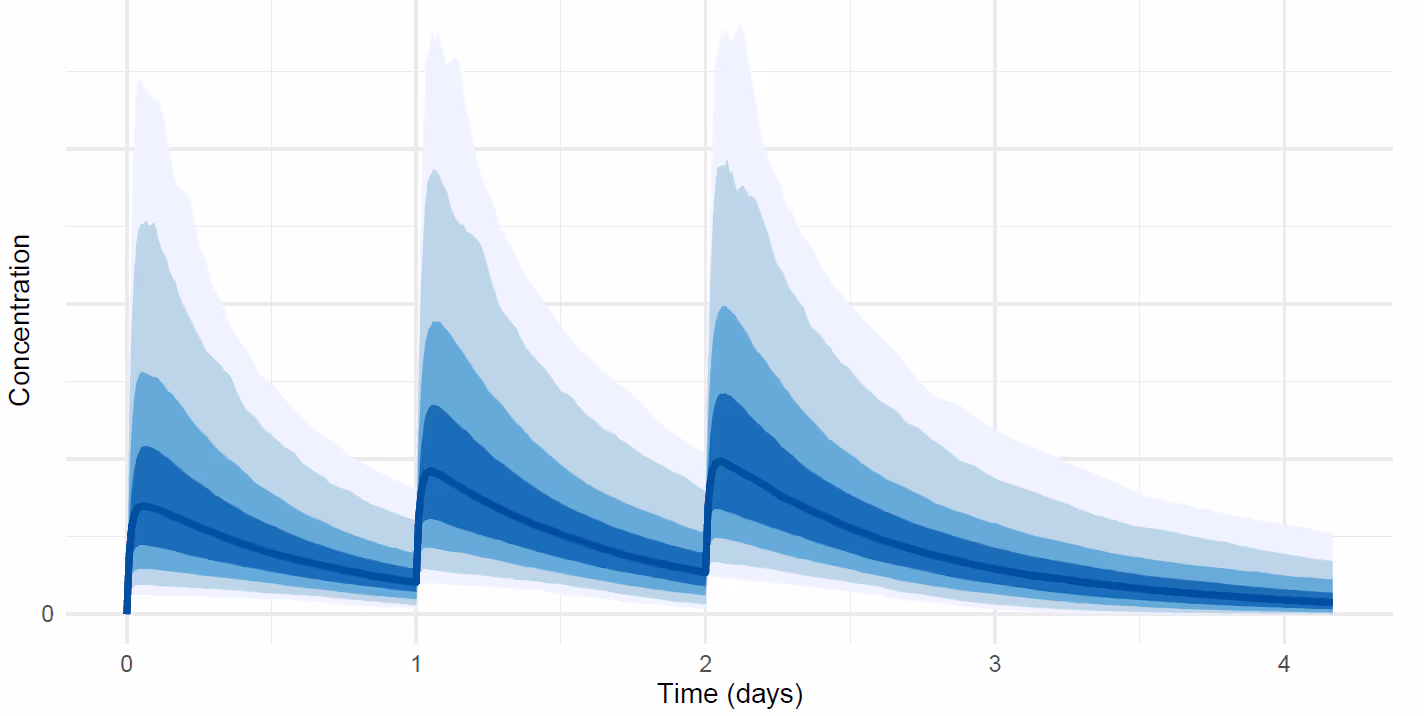
The full probabilistic model specifies probability distribution for the noise parameter $\sigma$ and other unknown parameters $\theta$. The function $\mu(t \mid \theta)$ would typically be deterministic given the values of $\theta$, such as in pharmacokinetic modeling or parametric tumor size modeling.
The above figure is an example visualization of a probability distribution of drug concentration that depends on time. For example the dark blue shading at each time point is the interval where the measurement lies with 50% probability, and the lightest blue shading is the interval where it lies with 95% probability. Probabilistic inferences such as these have more information than a single point-estimate fit without uncertainty. This type of model allows us to compute probabilistic inferences about derived quantities that are not directly measurable. For example, we can infer that "the half-life of the drug is greater than 3 months with 90% probability" or "the drug reduces tumor size by half with 40% probability when given X mg dose ."
By quantifying uncertainty, we can make smarter choices. Probabilistic inferences are useful in decision-making, which can be based on expected utilities of different decisions. Examples include choosing recommended doses based on patients preferences for certain types of risks or whether to advance the drug from Phase II to Phase III.
The above example was presented for a single imaginary patient. In reality, the studies that we analyze involve 10s to 1000s of subjects for whom we typically know some predictive characteristics such as age and treatment. The challenge is to set up the probabilistic model jointly for all unknowns so that the distributions of the measurements are correlated over subjects and depend on the predictive variables. This way we can, for instance, estimate the effect of a drug for a new yet unseen patient. The probabilistic models we use are typically joint models of multiple types of time-course data, such as drug concentration, adverse events, and biomarker measurements.
This is a comment related to the post above. It was submitted in a form, formatted by Make, and then approved by an admin. After getting approved, it was sent to Webflow and stored in a rich text field.
This is a comment related to the post above. It was submitted in a form, formatted by Make, and then approved by an admin. After getting approved, it was sent to Webflow and stored in a rich text field.
This is a comment related to the post above. It was submitted in a form, formatted by Make, and then approved by an admin. After getting approved, it was sent to Webflow and stored in a rich text field.
This is a comment related to the post above. It was submitted in a form, formatted by Make, and then approved by an admin. After getting approved, it was sent to Webflow and stored in a rich text field.
This is a comment related to the post above. It was submitted in a form, formatted by Make, and then approved by an admin. After getting approved, it was sent to Webflow and stored in a rich text field.
This is a comment related to the post above. It was submitted in a form, formatted by Make, and then approved by an admin. After getting approved, it was sent to Webflow and stored in a rich text field.
This is a comment related to the post above. It was submitted in a form, formatted by Make, and then approved by an admin. After getting approved, it was sent to Webflow and stored in a rich text field.
This is a comment related to the post above. It was submitted in a form, formatted by Make, and then approved by an admin. After getting approved, it was sent to Webflow and stored in a rich text field.
This is a comment related to the post above. It was submitted in a form, formatted by Make, and then approved by an admin. After getting approved, it was sent to Webflow and stored in a rich text field.
This is a comment related to the post above. It was submitted in a form, formatted by Make, and then approved by an admin. After getting approved, it was sent to Webflow and stored in a rich text field.
This is a comment related to the post above. It was submitted in a form, formatted by Make, and then approved by an admin. After getting approved, it was sent to Webflow and stored in a rich text field.
This is a comment related to the post above. It was submitted in a form, formatted by Make, and then approved by an admin. After getting approved, it was sent to Webflow and stored in a rich text field.
This is a comment related to the post above. It was submitted in a form, formatted by Make, and then approved by an admin. After getting approved, it was sent to Webflow and stored in a rich text field.
This is a comment related to the post above. It was submitted in a form, formatted by Make, and then approved by an admin. After getting approved, it was sent to Webflow and stored in a rich text field.
This is a comment related to the post above. It was submitted in a form, formatted by Make, and then approved by an admin. After getting approved, it was sent to Webflow and stored in a rich text field.
This is a comment related to the post above. It was submitted in a form, formatted by Make, and then approved by an admin. After getting approved, it was sent to Webflow and stored in a rich text field.
This is a comment related to the post above. It was submitted in a form, formatted by Make, and then approved by an admin. After getting approved, it was sent to Webflow and stored in a rich text field.
This is a comment related to the post above. It was submitted in a form, formatted by Make, and then approved by an admin. After getting approved, it was sent to Webflow and stored in a rich text field.
This is a comment related to the post above. It was submitted in a form, formatted by Make, and then approved by an admin. After getting approved, it was sent to Webflow and stored in a rich text field.
This is a comment related to the post above. It was submitted in a form, formatted by Make, and then approved by an admin. After getting approved, it was sent to Webflow and stored in a rich text field.
This is a comment related to the post above. It was submitted in a form, formatted by Make, and then approved by an admin. After getting approved, it was sent to Webflow and stored in a rich text field.
This is a comment related to the post above. It was submitted in a form, formatted by Make, and then approved by an admin. After getting approved, it was sent to Webflow and stored in a rich text field.
This is a comment related to the post above. It was submitted in a form, formatted by Make, and then approved by an admin. After getting approved, it was sent to Webflow and stored in a rich text field.
This is a comment related to the post above. It was submitted in a form, formatted by Make, and then approved by an admin. After getting approved, it was sent to Webflow and stored in a rich text field.
This is a comment related to the post above. It was submitted in a form, formatted by Make, and then approved by an admin. After getting approved, it was sent to Webflow and stored in a rich text field.
This is a comment related to the post above. It was submitted in a form, formatted by Make, and then approved by an admin. After getting approved, it was sent to Webflow and stored in a rich text field.
This is a comment related to the post above. It was submitted in a form, formatted by Make, and then approved by an admin. After getting approved, it was sent to Webflow and stored in a rich text field.

Trying to cut corners to make nonlinear PK model fitting faster
.svg)


This is a comment related to the post above. It was submitted in a form, formatted by Make, and then approved by an admin. After getting approved, it was sent to Webflow and stored in a rich text field.