
In the past, I’ve often not included priors in my models. I often felt daunted by having to pick sensible priors for my parameters, and I usually fell into the common trap of thinking that no priors or uniform priors are somehow the most objective prior because they “let the data do all the talking.” Recent experiences and have completely changed my thinking on this though.
Choosing good priors not only forces you to understand the intuitive meaning behind your model and its parameters, but it also can also help speed up your sampling algorithms, like HMC and NUTS, tremendously! Here, sampling refers to getting draws from your posterior distribution proportional to how probable they are. This is important because all Bayesian inference happens through the posterior distribution, a distribution over our unknown parameters that brings together our domain knowledge in the priors and the knowledge about the unknown parameters that the actual data, or experiments, provide.
So how do you choose good priors that won’t “bias” your fit? Well, as I’ll show, with a little thinking and practice it’s not that hard. It turns out we ALWAYS have some prior information about our unknown parameters. If you don’t believe me, there is a quote by Andrew Gelman that might make this more apparent. The quote was a rhetorical question something along the lines of “do you really believe your variance parameter can be anywhere from zero to infinity with equal probability?”
The answer to this is of course, “no, I don’t believe that.” I know the standard error of my measurement noise won’t be infinitely large, otherwise my data would be worthless noise and I wouldn’t be doing the analysis in the first place! If I’m modeling drug absorption, I know the parameter that controls absorption isn’t infinitely large because I know drugs don’t get absorbed instantly in the digestive system. So why should we consider ridiculously small or large values when we know they’re not possible?!
This week I’m going to walk through building and fitting a Stan model for the famous theophylline drug dataset. I show how not specifying priors in our models can be insensible, but how this is only apparent when we start caring about uncertainty intervals and move from optimization to sampling. I also mention a few traditional non-Bayesian techniques for obtaining uncertainty information about our estimates and some of the disadvantages they pose versus Bayesian sampling. I’ll show step-by-step how easy it is to choose priors that rule out nonsensical parameter values, even when you have minimal domain knowledge. Lastly, I’ll show a clever trick in Stan related to the prior-predictive distribution, that helps make choosing priors even easier and more intuitive, and I’ll show how all of this leads to fast, robust model estimation!
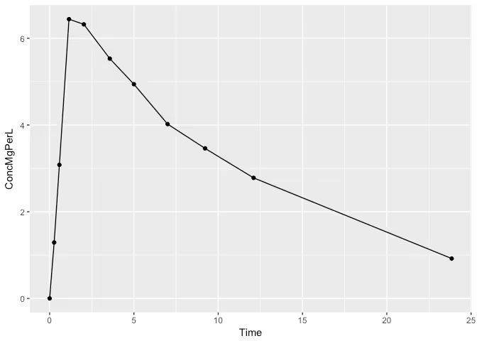
Most of us in the pharmacokinetic community are familiar with the theophylline dataset. The data comes from an experiment where 12 patients were dosed with a specific amount of the drug theophylline, a drug used to treat respiratory diseases such asthma. The data consists of measurements of the drugs concentration in the body over time for each patient, but for this blog post we’ll just be considering patient one. The dataset is available in the PKPDmodels package, so let’s take a peek!

The drug is taken orally and enters the digestive system at which point absorption in to the blood begins. Once in the blood, the drug begins to be cleared out by the body causing the peak and eventual decay we’re seeing in the plot above.
This phenomenon is often modeled by a two-compartment ordinary differential equation (ODE). The first compartment, $A_1$, represents the amount of the drug in the digestive system and the second compartment, $A_2$, represents the amount of the drug in the blood. The drug leaves the digestive system at a rate proportional to the amount in the digestive system and the drug leaves the blood at a rate proportional to the amount in the blood. In mathematical terms we have the following ODE, referred to in the pharmacokinetics literature as the “open one-compartment model with first order absorption” (Wang 2015):
$$\begin{align}
\frac{dA_1}{dt} &= -K_a A_1 \\
\frac{dA_2}{dt} &= K_a A_1 - K_e A_2
\end{align}$$
Here, Ka is a constant (to be estimated) that represents how fast the drug gets absorbed in to the blood stream and Ke is a constant that represents how fast the drug is eliminated from the blood.
At this point we can throw this in to Stan and start inferring those parameters from the data thanks to Stan’s built in ODE solvers. However, when the analytical solution is known it is preferred over having to solve the system numerically, as this will speed up our computational inference. In this case, the ODE is simple enough that we can solve for the analytical solution giving us the amount of the drug over time in the second compartment (Wang 2015):
$$A_2(t) = \frac{D K_a F}{K_a - K_e} \left( \exp(-K_e t) - \exp(-K_a t) \right)$$
Here, D is the dose amount in milligrams and F is a fraction between zero and one called the bioavailability which represents how much of the drug the body actually absorbs. This term is there because some of the drug gets destroyed by stomach acids or doesn’t make it in to the blood for a plethora of reasons.
Note that we only need the solution to the second compartment because that’s the only compartment we observe concentrations in. Once we solve for the amount, it’s easy to obtain the concentration by dividing by the volume of distribution, $V_d$, another parameter to be estimated.
Armed with our mechanistic model of the drug concentration we’re ready to build a statistical model to explain our data.
Let’s start by specifying our data in Stan. We have a dose amount, observations of drug concentration over time, and the time points they were observed at:
data {
  real<lower = 0> dose;
  int<lower = 0> N_obs;
  vector[N_obs] obs_times;
  real<lower = 0> obs[N_obs];
}
Next we have our parameters that we’d like to estimate. Note the lower bounds on $K_e$ and $K_a$. The reason for this is that we know from looking at the analytical solution that KaKa must be greater than $K_e$ otherwise we’d get a negative concentration which is impossible! The other parameters are constrained to be positive of course, and the bioavailability factor is constrained to be between zero and one.
parameters {
  real<lower = 0, upper = 1> F;  // bioavailability factor
  real<lower = 0> Ke;            // Ke must be greater than 0
  real<lower = Ke> Ka;           // Ka must be greater than Ke
  real<lower = 0> Vd;            // volume of distribution
  real<lower = 0> sigma;         // size measurement error
}
In Stan we can specify a transformed parameters block which consists of quantities we’d like to estimate and use in our model that are strictly a function of the parameters. This is useful, for example, when we’d like to track samples of the mean concentration levels of the drug.
transformed parameters {
  vector[N_obs] C;

  real theta[3] = {F, Ka, Ke};
  C = OneComparmentAmountAnalytic(obs_times, dose, theta) / Vd + 1e-3;
}
The function to compute the analytic solution can be defined at the top of the Stan model as follows:
functions {
  vector OneComparmentAmountAnalytic(vector t, real D, real[] theta) {
    int T = num_elements(t);

    real F = theta[1];
    real Ka = theta[2];
    real Ke = theta[3];

    vector[T] A2 = (D * Ka * F) / (Ka - Ke) * (exp(-Ke * t) - exp(-Ka * t));

    return A2;
  }
}
Lastly, we can specify our statistical model, which in this case will be pretty simple. Since this post is all about priors, let’s start by not including any priors on our parameters just to see what happens!
model {
  obs ~ lognormal(log(C), sigma);
}
Now that we’ve written our model in Stan, we’re ready to fit our unknown parameters to the data! The most basic approach to doing this is maximum likelihood estimation. Essentially we have a likelihood function, $\mathcal{L}(F, K_e, K_a, V_d, \sigma \mid D)$, that we plug our data, $D$ in to. From there, we can evaluate how “likely” different combinations of the parameters are given our data. Maximum likelihood estimation, as one would imagine, just involves trying different parameters and plugging them in to the likelihood function until you find one that seems the most likely. Geometrically, our likelihood function can be thought of as a surface: a function over parameter space that assigns a single value to each point in parameter space. Imagined this way, we just want to find the maximum of this surface.
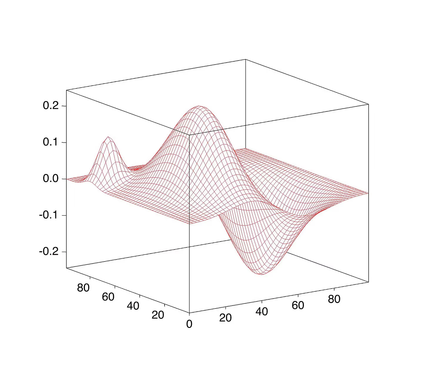
Let’s compile our model and do this in Stan! All we need to do is provide our data and an initial point in parameter space to try, and Stan’s optimization algorithm will keep climbing up the surface until it has reached a peak.
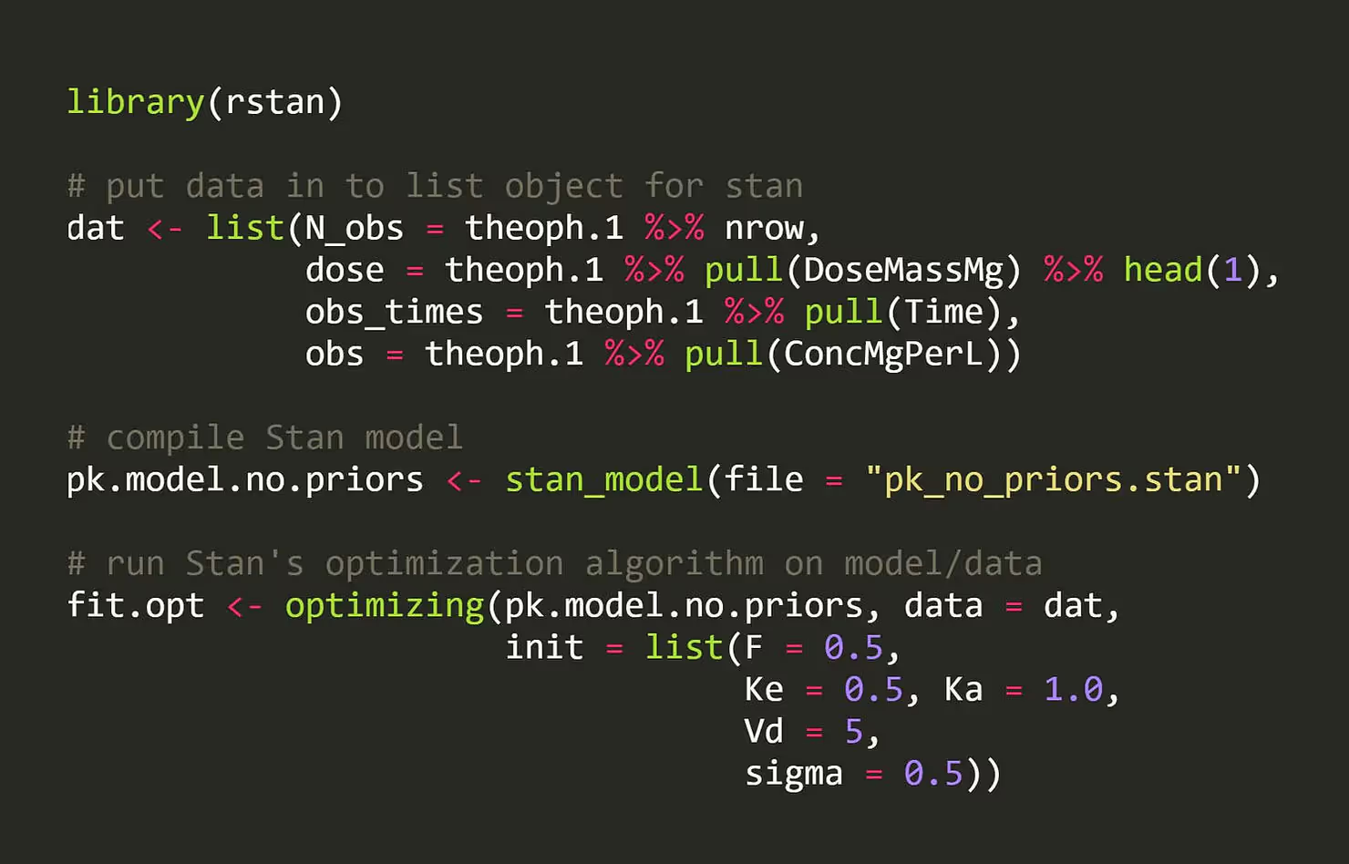
Great! Let’s check out the maximum likelihood estimates!

## # A tibble: 1 x 5
##       F    Ka     Ke    Vd sigma_sq
##   <dbl> <dbl>  <dbl> <dbl>    <dbl>
## 1 0.408 0.915 0.0945  17.0   0.0172
We can also check the expected value of the concentration curve a the times where we observed data (the red is the true data and the blue is the maximum-likelihood estimated trajectory):

## Warning: attributes are not identical across measure variables;
## they will be dropped
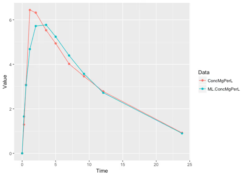
Not bad! Maximum likelihood optimization gives us a likely value of what our parameters might be, and it even leads to sensible concentration curves, but how certain can we be that these likely values are close to the truth? I mean if we’re testing drugs in a patient we probably don’t want to get this (too) wrong, right?
While optimization tries to find a single value of our parameter that explains the fit, sampling essentially gives us multiple possible values that could explain our fit in proportion to how well each one explains. In this way we can quantify how uncertain we are about our parameter estimate.
Why is it important to consider all the possibilities? Data is always noisy and maximum likelihood estimates are a function of our data, so if we’re unlucky we get a misleading maximum likelihood estimate. If the parameter is say how fast a drug gets cleared from the system, it’s good to know what’s the highest it can be, lest we give someone too much of a drug.
As an aside, it turns out that if you’re trying to estimate many parameters at once, like say ten or more, and you don’t have a lot of data, not only MIGHT your maximum likelihood not be representative of the true values, it probably WON’T be representative of the true values. Look up Michael Betancourt’s YouTube videos on Concentration of Measure for more on this somewhat counter-intuitive fact.
As another aside, not all statisticians use sampling to quantify uncertainty in their estimates. Some statisticians like to prove that their maximum likelihood estimator will have a high chance of being close to the true value of the parameters if one had infinite data (consistency). Others, like to show mathematically that their maximum likelihood estimator starts to look normally distributed once they use enough data. If you had to take a statistics qualifying exam at one point in your life, this stuff is permanently etched in your memory. The problem with these techniques however is that we don’t have infinite data and it’s hard to say how much is close enough to infinite!
Still others, resample from their data, essentially simulating a rerun of the experiment, and then obtain a separate maximum likelihood estimate for each “resampled” dataset. They then examine the values of all the maximum likelihood estimates they computed on each simulated rerun. This is known as bootstrapping.
In Bayesian statistics, we don’t think about hypothetical reruns of our experiment. We only consider the experiment at hand, which consists of finite data. In fact, we don’t really take single estimates. All knowledge about our parameters is captures in the posterior distribution, which tells us what parameter values are possible given the data we’ve seen, how probable they are, and our uncertainty in the values of these parameters. This starts with quantifying our uncertainty regarding the parameters first in our prior distribution. This is to say that in Bayesian statistics we explicitly assign a distribution to the unknown parameters that captures our prior knowledge.
Quantifying our knowledge of our unknown parameters before seeing any data sounds scary! What if we choose the wrong distribution for our parameters, or our knowledge isn’t exactly reflected? Well we probably won’t be exactly right, just like we might choose the wrong model for our data, but as the common aphorism goes “all models are wrong, but some are useful.” We just have to be somewhat careful about how we choose that distribution which we call the prior, as I’ll illustrate. This is akin to being careful to ensure that your data really is Gaussian distributed when using OLS regression. One thing I really love about Bayesian statistics is that once you make this leap of faith to say unknown parameters follow a distribution you gain the power to easily write and fit elaborate multi-level models that would otherwise be difficult to fit or interpret (random effects models for you frequentists out there).
Now that we’ve talked all about uncertainty and sampling let’s actually do it with our Stan model! When we created our model, we specified our log-normal likelihood, and we implicitly put a uniform prior on our unknown parameters, by not including priors. This means that we believe all of our unknown parameters can be anywhere between zero and infinity with equal probability.
Using Bayes' rule and Stan’s NUTS sampler, we can now sample from our posterior distribution, i.e. the distribution of our parameters given the data:

##
## SAMPLING FOR MODEL 'pk_no_priors' NOW (CHAIN 1).
##
## Gradient evaluation took 2.2e-05 seconds
## 1000 transitions using 10 leapfrog steps per transition
## would take 0.22 seconds.
## Adjust your expectations accordingly!
##
##
## Iteration:    1 / 2000 [  0%]  (Warmup)
## Iteration:  200 / 2000 [ 10%]  (Warmup)
## Iteration:  400 / 2000 [ 20%]  (Warmup)
## Iteration:  600 / 2000 [ 30%]  (Warmup)
## Iteration:  800 / 2000 [ 40%]  (Warmup)
## Iteration: 1000 / 2000 [ 50%]  (Warmup)
## Iteration: 1001 / 2000 [ 50%]  (Sampling)
## Iteration: 1200 / 2000 [ 60%]  (Sampling)
## Iteration: 1400 / 2000 [ 70%]  (Sampling)
## Iteration: 1600 / 2000 [ 80%]  (Sampling)
## Iteration: 1800 / 2000 [ 90%]  (Sampling)
## Iteration: 2000 / 2000 [100%]  (Sampling)
##
##  Elapsed Time: 7.75569 seconds (Warm-up)
##                8.16377 seconds (Sampling)
##                15.9195 seconds (Total)
## Warning: There were 1000 transitions after warmup that exceeded
## the maximum treedepth. Increase max_treedepth above 10. See
## http://mc-stan.org/misc/warnings.html#maximum-treedepth-exceeded
## Warning: There were 1 chains where the estimated Bayesian Fraction of
## Missing Information was low. See
## http://mc-stan.org/misc/warnings.html#bfmi-low
## Warning: Examine the pairs() plot to diagnose sampling problems
Hmm, warnings from Stan. That’s often a sign that something is wrong with our posterior, and we that we can’t trust our samples. We can look at a pairs plots of our posterior samples to ge a better idea of what’s going on.

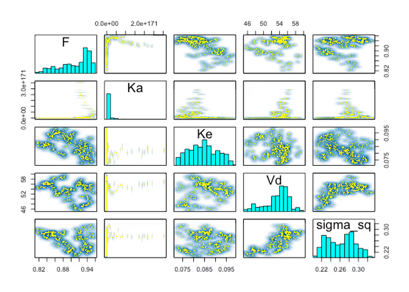
Woah! We’re sampling all kind of crazy values, like absorption rates that are greater than 4e1774e177! As a rule of thumb, the number of hours it takes for the 99% of the drug to be absorbed is (4.6/Ka)(4.6/Ka), which means we’re sampling values that imply the drug is absorbed nearly instantly. There’s no way an absorption rate that fast is possible. We know that it takes some time for the drug to get absorbed in the blood stream.
So what’s going on? Well, remember our likelihood surface that we were trying to optimize before? Now we’re actually exploring it using MCMC and Stan’s NUTS algorithms, instead of trying to find the peak of it. There are no guarantees that this surface isn’t bumpy or flat or has other ugly features, especially when we don’t include prior information.
Part of the reason the sampler tried a value for Ka as high as 4e1774e177 is because by not including a prior we implicitly made the assumption that 4e1774e177 is just as valid as a more reasonably value like say Ka=4Ka=4, which would imply the drug gets absorbed in about an hour.
Let’s include some meaningful priors that are actually consistent with what we believe and see what happens!
So first things first: how do we insert meaningful priors in to our models? Well, recall we’re trying to estimate five parameters: F,Ke,Ka,Vd,F,Ke,Ka,Vd, and σσ. FF is the bioavailability factor, which can be anywhere between zero and one. Thus a natural prior to place on it is the Beta distribution, a distribution on numbers between zero and one. The other parameters we know should be strictly positive, so a natural prior to use is the Log-Normal distribution, whose log is normally distributed (nice naming right?).
Now how do we incorporate our knowledge, or in this case my knowledge, about these parameters in our model? Let’s walk through it!
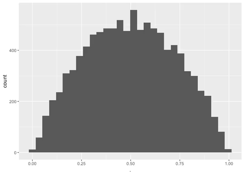
I don’t know much about the bioavailability factor of this drug, FF. We can just use a Beta(1,1)Beta(1,1) prior which is uniform on zero to one, although that is somewhat conservative, as I know that no oral drug gets perfectly absorbed and I know that if none if it got absorbed we wouldn’t be testing it. So let’s pick a Beta prior that avoids these extreme values, but still allows for them. This way if the data really suggests that these values are plausible, we’ll still infer that.

## `stat_bin()` using `bins = 30`. Pick better value with `binwidth`.
Next let’s consider the absorption rate, KaKa. Well in this case I know that a pill will reach the stomach and start breaking then go to the small intestine where it may be absorbed and this could happen on the scale of minutes to hours. I also know from a quick Google search that digestion takes about 6 to 8 hours. So really we know that most of the drug can be absorbed anywhere from a few minutes to say 12 hours, but we’ll be conservative and say it might take 24 hours. Now we just have to find appropriate parameters for a Log-Normal distribution that captures this knowledge. For this I recommend getting intimate with your basic distributions by drawing from them in R and plotting histograms. In this case I’ll draw possible values of Ka then divide \4.6\) by these values so that I can get the actually 99% absorption times these prior values lead to.

## `stat_bin()` using `bins = 30`. Pick better value with `binwidth`.
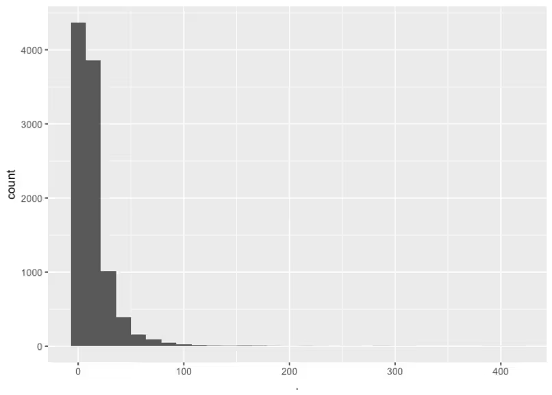
This prior puts most of the weight on values smaller than 24 hours, and most before 12. This prior allows for values which could possibly result in a 99% absorption time of over 100, which probably isn’t possible, but that’s ok, we’ll be conservative. As long as we’re not considering absurd values like 4e177 like we were doing before.
As for the elimination rate Ke, we know it should be smaller than Ka, but let’s just be conservative and give it the same distribution.
Now the volume of distribution, Vd, is a specific parameter used in PK modeling that varies for different drugs. Intuitively, it should represent the volume of liquid in the body a drug has access to, but not quite. In fact, it’s sort of hard to interpret as a physical value. Luckily the fantastic book (Rosenbaum 2016) provides a neat table I took a picture of with values of Vd parameters for various drugs. This give us an idea of what we could expect.
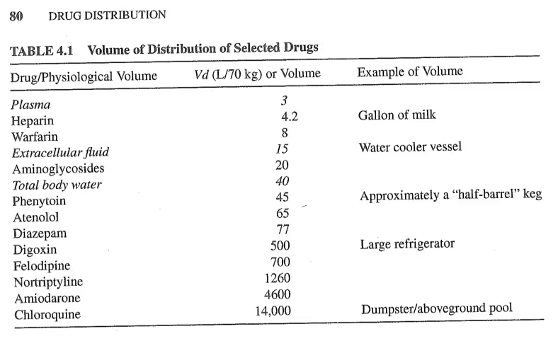
These values range mostly in the dozens, with one drug reaching up to 14,000. I’m not sure how extreme or realistic that actually is, but let’s be conservative and set a prior with most of its mass under a thousand, but that still have some mass uniformly up to 14,000. Again, usually you want to play around this these distributions by randomly sampling from them, but for brevity I’m just showing samples for my final choice.

## `stat_bin()` using `bins = 30`. Pick better value with `binwidth`.
## Warning: Removed 2804 rows containing non-finite values (stat_bin).
## Warning: Removed 2 rows containing missing values (geom_bar).
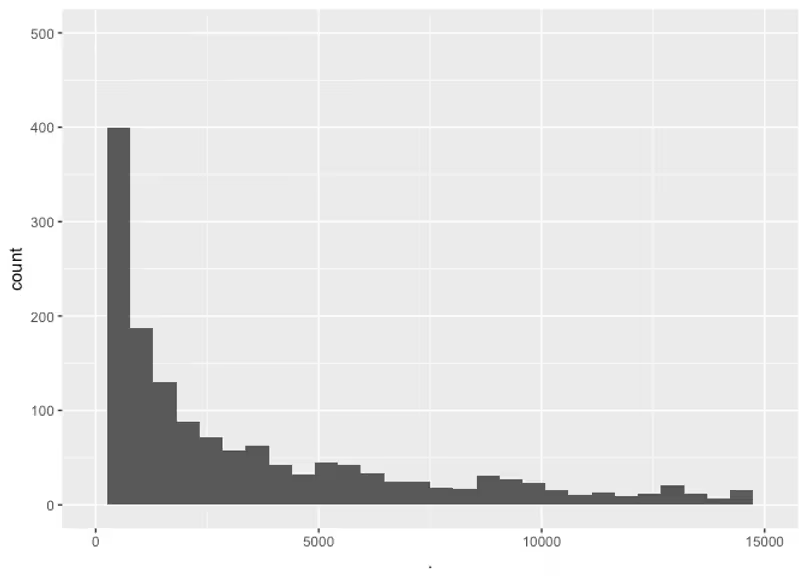
This way we’re representing our knowledge that most of the time the VdVd is under a thousand, but we’re not ruling out the possibility of it being much higher in the ten thousands. If the data really provides evidence for this parameter being that high, we should see it after we fit.
Lastly, we must pick a prior for the σσ parameter which represents the standard error of our observations on the log scale. For this, let’s have a look at our data again on the log scale.

##  [1] -6.90775528  0.25541711  1.12525422  1.86268381  1.84387742
##  [6]  1.71036863  1.59756774  1.39153063  1.24155756  1.02281058
## [11] -0.08229524
Since on the log scale, most of our observations are around 1.0 it’s reasonable to assume that if our measurements aren’t too extremely noisy, the standard error should be around 0.1 but no more than 1 and or 2. It’s unrealistic to expect any more than that because that would mean our measurements are so noisy as to not be informative of anything. Again, we’ll be conservative and go with a LogNormal(0,1.0) prior, which puts most of its mass below five.
Putting this all together in to our Stan model we have the following:
model {
  // prior
  F ~ beta(1, 1);
  Ka ~ lognormal(-0.6, 1);
  Ke ~ lognormal(-0.6, 1);
  Vd ~ lognormal(log(40), 10);
  sigma ~ lognormal(0, 1);

  // likelihood
  obs ~ lognormal(log(C), sigma);
}
Now with our priors that rule out nonsensical values we’re ready to get back to sampling the posterior distribution. Before we do that I think it’s worth it to mention another cool technique I recently learned that makes choosing your prior distributions even more intuitive when you have complicated models. The technique involves sampling from what’s called the prior-predictive distribution.
Basically if we have something like an ODE or other complicated model that depends on unknown parameters, we sample from our the priors of those unknown parameters and we see if we get reasonable ODE solutions or other reasonable values of our observations. This turns out to be an extremely powerful tool and is what Bayesian generative modeling is all about: once we set up a model of the process that we believe describes our data/experiment, then we can generate synthetic data from our model to see if our model is reasonable.
We can do this in Stan by making a simple modification to our code. We take our likelihood, which is what ties together our data and unknown parameters, and wrap it in an if statement so that we can take it out of our model so that we’re only taking draws from the prior in Stan:
model {
  // prior
  F ~ beta(1, 1);
  Ka ~ lognormal(-0.6, 1);
  Ke ~ lognormal(-0.6, 1);
  Vd ~ lognormal(log(40), 10);
  sigma ~ lognormal(0, 1);

  // likelihood
  if (!posterior_predictive) {
    obs ~ lognormal(log(C), sigma);
  }
}
Now when we run our model we can take draws from our prior distribution and see what kinds of ODE solutions these priors actually manifest as. Here I sample from our model with the likelihood off, and I get 10% to 90% uncertainty intervals for the drug concentration level at the points where we observed data for our patient. To give us an idea of how reasonable these “generated” concentration values are, I overlay the actual concentration values we have in our data.

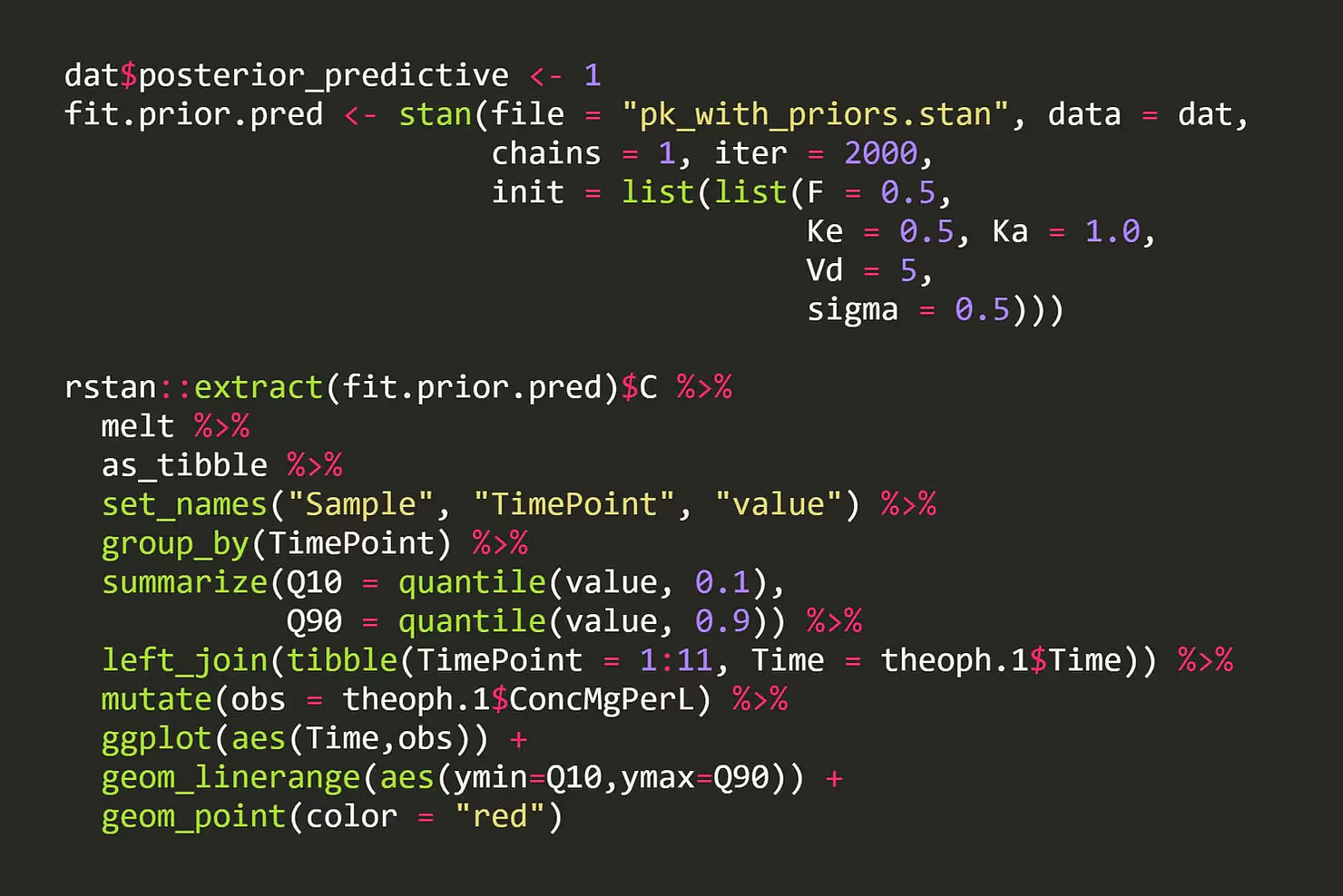
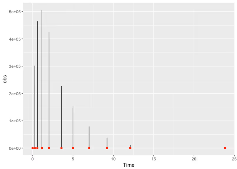
Woah! What our generative model is telling us here is that our priors are allowing for concentration curves that are several ordered of magnitude above what we should reasonably expect. This tells us that we can improve our priors. Remember our Vd parameter that we said was probably in the dozens, but that we gave a prior that allowed for a value in the tens of thousands? Let’s tighten that up to something more reasonable and see what happens.

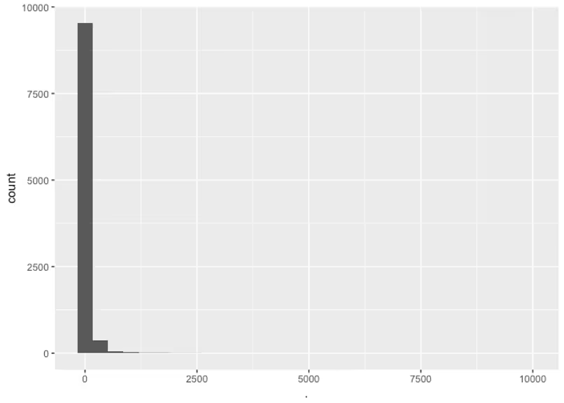
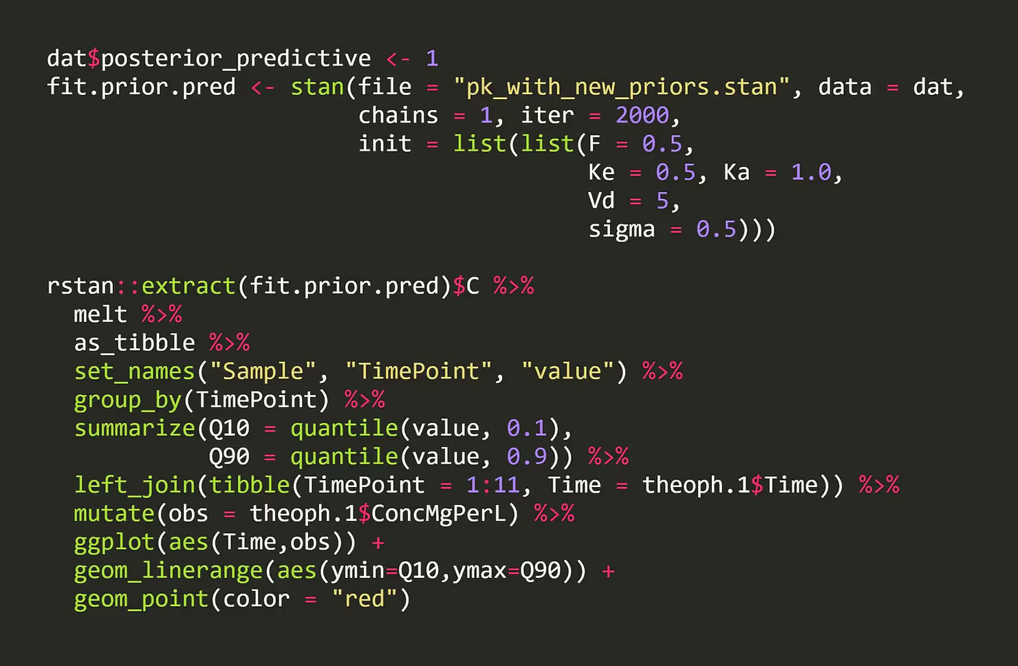

Now our priors are leading to possible concentration curves that are much more sensible. We’ve successfully included our priors knowledge in our model, and we didn’t have to be pharmacology experts!
Let’s turn our likelihood back on and see how everything fits now.


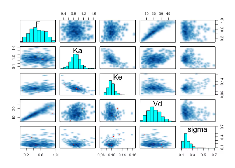
First off there’s no warnings from Stan, and the pairs plots are looking smooth and sensible. That’s a good sign. Let’s check out what kinds of solutions we’re sampling now that we’re actually incorporating the data.
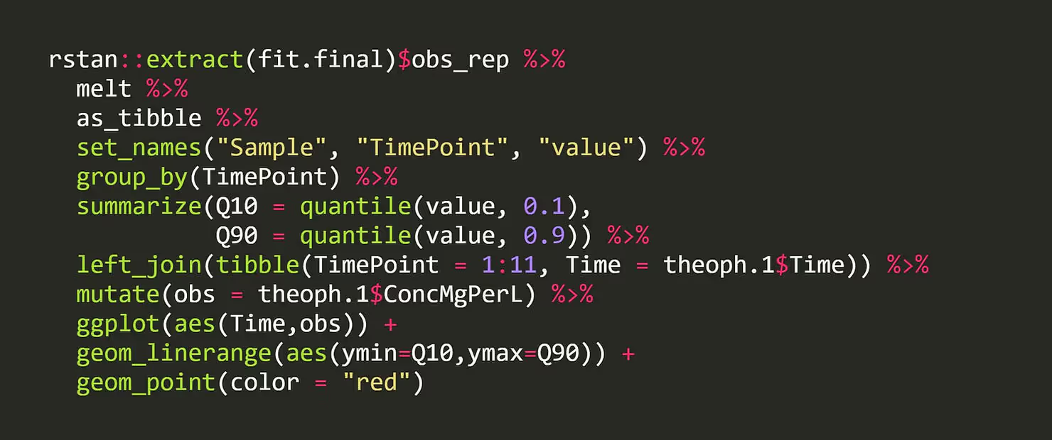
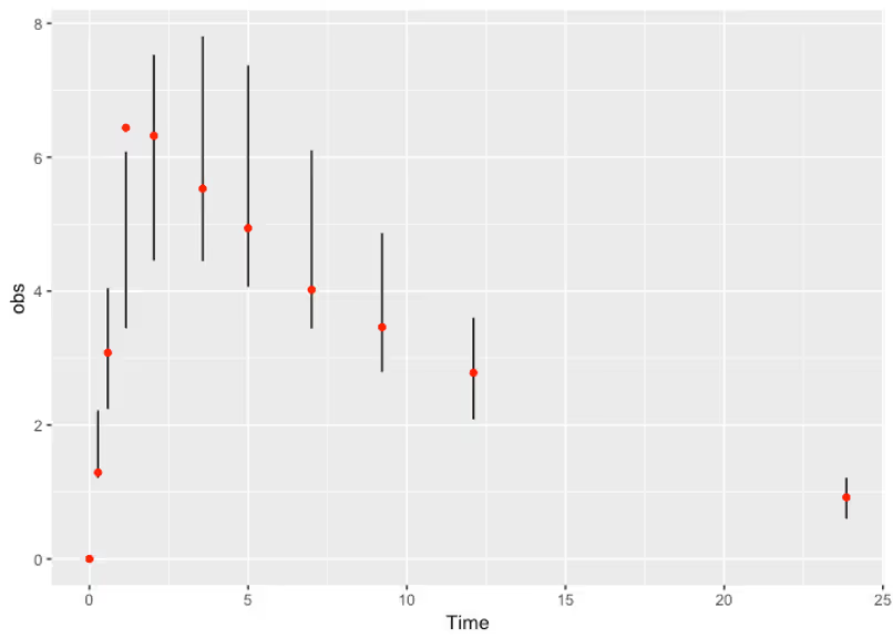
Nice! Lastly we’ll take a look at the posterior quantiles of our parameters. In practice these give us an idea of how fast we should expect the drug to be absorbed or cleared from the body.

## Inference for Stan model: pk_with_new_priors.
## 1 chains, each with iter=2000; warmup=1000; thin=1;
## post-warmup draws per chain=1000, total post-warmup draws=1000.
##
##        mean se_mean   sd 2.5%   25%   50%   75% 97.5% n_eff Rhat
## F      0.50    0.01 0.20 0.14  0.35  0.49  0.67  0.89   283    1
## Ka     0.88    0.01 0.20 0.48  0.76  0.88  1.00  1.33   262    1
## Ke     0.10    0.00 0.01 0.07  0.09  0.10  0.11  0.13   206    1
## Vd    20.27    0.50 8.48 6.00 14.11 19.52 26.23 38.29   282    1
## sigma  0.21    0.01 0.08 0.12  0.16  0.19  0.23  0.45   183    1
##
## Samples were drawn using NUTS(diag_e) at Thu Jul 19 15:44:15 2018.
## For each parameter, n_eff is a crude measure of effective sample size,
## and Rhat is the potential scale reduction factor on split chains (at
## convergence, Rhat=1).
Rosenbaum, Sara E. 2016. Basic Pharmacokinetics and Pharmacodynamics: An Integrated Textbook and Computer Simulations. John Wiley & Sons.
Wang, Jixian. 2015. Exposure–Response Modeling: Methods and Practical Implementation. Chapman; Hall/CRC.
This is a comment related to the post above. It was submitted in a form, formatted by Make, and then approved by an admin. After getting approved, it was sent to Webflow and stored in a rich text field.
This is a comment related to the post above. It was submitted in a form, formatted by Make, and then approved by an admin. After getting approved, it was sent to Webflow and stored in a rich text field.
This is a comment related to the post above. It was submitted in a form, formatted by Make, and then approved by an admin. After getting approved, it was sent to Webflow and stored in a rich text field.
This is a comment related to the post above. It was submitted in a form, formatted by Make, and then approved by an admin. After getting approved, it was sent to Webflow and stored in a rich text field.
This is a comment related to the post above. It was submitted in a form, formatted by Make, and then approved by an admin. After getting approved, it was sent to Webflow and stored in a rich text field.
This is a comment related to the post above. It was submitted in a form, formatted by Make, and then approved by an admin. After getting approved, it was sent to Webflow and stored in a rich text field.
This is a comment related to the post above. It was submitted in a form, formatted by Make, and then approved by an admin. After getting approved, it was sent to Webflow and stored in a rich text field.
This is a comment related to the post above. It was submitted in a form, formatted by Make, and then approved by an admin. After getting approved, it was sent to Webflow and stored in a rich text field.
This is a comment related to the post above. It was submitted in a form, formatted by Make, and then approved by an admin. After getting approved, it was sent to Webflow and stored in a rich text field.
This is a comment related to the post above. It was submitted in a form, formatted by Make, and then approved by an admin. After getting approved, it was sent to Webflow and stored in a rich text field.
This is a comment related to the post above. It was submitted in a form, formatted by Make, and then approved by an admin. After getting approved, it was sent to Webflow and stored in a rich text field.
This is a comment related to the post above. It was submitted in a form, formatted by Make, and then approved by an admin. After getting approved, it was sent to Webflow and stored in a rich text field.
This is a comment related to the post above. It was submitted in a form, formatted by Make, and then approved by an admin. After getting approved, it was sent to Webflow and stored in a rich text field.
This is a comment related to the post above. It was submitted in a form, formatted by Make, and then approved by an admin. After getting approved, it was sent to Webflow and stored in a rich text field.
This is a comment related to the post above. It was submitted in a form, formatted by Make, and then approved by an admin. After getting approved, it was sent to Webflow and stored in a rich text field.
This is a comment related to the post above. It was submitted in a form, formatted by Make, and then approved by an admin. After getting approved, it was sent to Webflow and stored in a rich text field.
This is a comment related to the post above. It was submitted in a form, formatted by Make, and then approved by an admin. After getting approved, it was sent to Webflow and stored in a rich text field.
This is a comment related to the post above. It was submitted in a form, formatted by Make, and then approved by an admin. After getting approved, it was sent to Webflow and stored in a rich text field.
This is a comment related to the post above. It was submitted in a form, formatted by Make, and then approved by an admin. After getting approved, it was sent to Webflow and stored in a rich text field.
This is a comment related to the post above. It was submitted in a form, formatted by Make, and then approved by an admin. After getting approved, it was sent to Webflow and stored in a rich text field.
This is a comment related to the post above. It was submitted in a form, formatted by Make, and then approved by an admin. After getting approved, it was sent to Webflow and stored in a rich text field.
This is a comment related to the post above. It was submitted in a form, formatted by Make, and then approved by an admin. After getting approved, it was sent to Webflow and stored in a rich text field.
This is a comment related to the post above. It was submitted in a form, formatted by Make, and then approved by an admin. After getting approved, it was sent to Webflow and stored in a rich text field.
This is a comment related to the post above. It was submitted in a form, formatted by Make, and then approved by an admin. After getting approved, it was sent to Webflow and stored in a rich text field.

Weighing pros and cons of NCA vs. PK modeling.

This is a comment related to the post above. It was submitted in a form, formatted by Make, and then approved by an admin. After getting approved, it was sent to Webflow and stored in a rich text field.