

Today, it seems like everyone is an epidemiologist. I am definitely not an epidemiologist but I did want to learn the basics of the popular SIR (Susceptible, Infected, Recovered) models. My guide is “Contemporary statistical inference for infectious disease models using Stan” by Chatzilena et al. [1], which does a great job at describing the model and in the spirit of reproducibility provides both Stan and R code. In this blog post, I will test a slightly modified version of the model on a simulated dataset and implement out-of-sample prediction logic in Stan.
The SIR model can be formulated using a three-state ODE system as follows.
$$\begin{align*}
\frac{\text{d}S}{\text{d}t} &= -\beta \frac{I(t)}{N} S(t) \\
\frac{\text{d}I}{\text{d}t} &= \beta \frac{I(t)}{N} S(t) - \gamma I(t) \\
\frac{\text{d}R}{\text{d}t} &= \gamma I(t)
\end{align*}$$
$S(t)$ is the number of susceptible individuals, $I(t)$ is infected, and $R(t)$ is recovered. $N$ is the total population which is the sum of the three groups, $\beta$ represents the transmission rate, $\gamma$ the recovery rate, and the by now infamous $R_0$, the basic reproduction number is the ratio $\beta / \gamma$. When $R_0 > 1$, in this model, the infection starts spreading in the population.
In case you are a pharmacometrician, this model has a multi-compartment flavor to it: the disease enters the susceptible population, reduces its size by infecting a fraction of people, and the infected fraction is reduced by the fraction of individuals who recover from the disease.
It is easy to set up a forward simulation from this model in R thanks to the deSolve package that implements a number of ODE solvers.
library(ggplot2)
library(deSolve)
library(tidyr)
theme_set(theme_minimal())

# S: susceptible, I: infected, R: recovered
SIR <- function(t, state, pars) {
  with(as.list(c(state, pars)), {
    N <- S + I + R
    dS_dt <- -b * I/N * S
    dI_dt <-  b * I/N * S - g * I
    dR_dt <-  g * I
    return(list(c(dS_dt, dI_dt, dR_dt)))
  })
}
Once the ODE system is set up, we pick the values for the parameters, initial conditions, and times points and use the solver. I took the population size and estimated parameter values from the paper:
In 1978, there was a report to the British Medical Journal for an influenza outbreak in a boarding school in the north of England. There were 763 male students which were mostly full boarders and 512 of them became ill.
n <- 100
n_pop <- 763
pars <- c(b = 2, g = 0.5)
state <- c(S = n_pop - 1, I = 1, R = 0)
times <- seq(1, 15, length = n)
sol <-
ode(
y = state,
times = times,
func = SIR,
parms = pars,
method = "ode45"
)
sol <- as.data.frame(sol)
sol_long <- sol |>
tidyr::pivot_longer(-time, names_to = "state", values_to = "value")
sol_long |>
ggplot(aes(time, value, color = state)) +
geom_line() +
guides(color = guide_legend(title = NULL)) +
scale_color_discrete(labels = c("Infected", "Recovered", "Susceptible")) +
xlab("Days") + ylab("Number of people") +
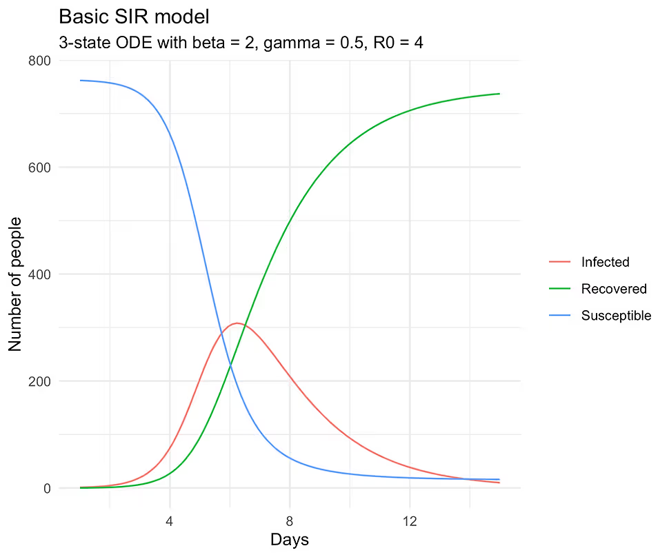
ggtitle("Basic SIR model", subtitle = "3-state ODE with beta = 2,
gamma = 0.5, R0 = 4")
If you run the above code, you should see the following plot:
Forward simulations are easy and fun but science works in the other direction. We observe noisy data, which in our case are diagnosed infections, and from these data and the stated model, we must learn all the plausible values of the parameters. To simulate the noisy data generating process, we will assume that our observed infections y are Poison distributed (not a great assumption, but will do for our purposes) with the rate $\lambda(t)$ equal to $I(t)$ from the solver.
set.seed(1234)
y <- rpois(n, sol$I)
The following Stan code is a slightly modified version of the one found in the paper. I changed the priors a bit, put some additional constraints on the parameters, and made the ODE code a little more readable. You will also notice that unlike in the forward simulation, the ODE in the Stan program is parameterized without the $1/N$ term. This is to ensure that the solution is on the proportion scale, which is converted back to the absolute scale when computing $\lambda(t)$ and later in the make_df() R function. Code listing can be accessed here [2].
functions {
  vector SIR(real t,vector y, array[] real theta) {
    real S     = y[1];
    real I     = y[2];
    real R     = y[3];

    real beta  = theta[1];
    real gamma = theta[2];

    vector[3] dydt;

    dydt[1] = -beta * S * I;
    dydt[2] =  beta * S * I - gamma * I;
    dydt[3] =  gamma * I;

    return dydt;
  }
}

data {
  int<lower=1> n_obs;   // number of observation times
  int<lower=1> n_pop;   // total population size
  array[n_obs] int y;   // observed infected counts
  real t0;              // initial time (e.g. 0)
  array[n_obs] real ts; // times at which y was observed
}

parameters {
  array[2] real<lower=0> theta; // {beta, gamma}
  real<lower=0,upper=1> S0;     // initial susceptible fraction
}

transformed parameters {
  vector[3] y_init;             // [S(0), I(0), R(0)]
  array[n_obs] vector[3] y_hat; // solution at each ts
  array[n_obs] real lambda;     // Poisson rates

  // set initial conditions
  y_init[1] = S0;
  y_init[2] = 1 - S0;
  y_init[3] = 0;

  y_hat = ode_rk45(SIR, y_init, t0, ts, theta);

  // convert infected fraction → expected counts
  for (i in 1:n_obs)
    lambda[i] = y_hat[i, 2] * n_pop;
}

model {
  theta ~ lognormal(0, 1);
  S0    ~ beta(1, 1);
  y     ~ poisson(lambda);
}

generated quantities {
  real R_0 = theta[1] / theta[2];
}
Once the Stan model is ready, we can construct the input dataset and start the sampling. I use the CmdStanR interface to run Stan which points to CmdStan on your computer (it needs to be installed separately; installation instruction here.)
library(cmdstanr)
library(posterior)

data <- list(n_obs = n, n_pop = n_pop, y = y, t0 = 0, ts = times)
sir_mod <- cmdstan_model("sir.stan")
sir_fit <- sir_mod$sample(
  data = data,
  seed = 1234,
  chains = 4,
  parallel_chains = 4,
  iter_warmup = 500,
  iter_sampling = 500
)

theta <- as_draws_rvars(sir_fit$draws(variables = "theta"))
We check convergence and see if we recover our parameter values for $\beta = \text{theta[1]}$ and $\gamma = \text{theta[2]}$:
> summarise_draws(theta, default_convergence_measures())
# A tibble: 2 × 4
  variable  rhat ess_bulk ess_tail
  <chr>    <dbl>    <dbl>    <dbl>
1 theta[1]  1.00     574.     779.
2 theta[2]  1.00     993.     932.

summarise_draws(theta, ~ quantile(.x, probs = c(0.05, 0.5, 0.95)))
# A tibble: 2 × 4
  variable  `5%` `50%` `95%`
  <chr>    <dbl> <dbl> <dbl>
1 theta[1] 1.96  2.00  2.03
2 theta[2] 0.488 0.494 0.502
This looks good but I also want to see if we captured our infection curve. For that, we need to extract the y_hat and plot them against the true curve from the solver.
y_hat <- as_draws_rvars(sir_fit$draws(variables = "y_hat"))

# helper function used for plotting the results
make_df <- function(d, interval = .90, t, obs, pop) {
  S <- d$y_hat[, 1] # Susceptible draws, not used
  I <- d$y_hat[, 2] # Infected draws
  R <- d$y_hat[, 3] # Recovered draws, not used

  # compute the uncertainty interval
  low_quant <- (1 - interval) / 2
  high_quant <- interval + low_quant
  low <- apply(I, 2, quantile, probs = low_quant) * pop
  high <- apply(I, 2, quantile, probs = high_quant) * pop

  return(tibble(low, high, times = t, obs))
}

d <- make_df(d = y_hat, interval = 0.90, times, obs = sol$I, pop = n_pop)
ggplot(aes(times, obs), data = d) +
  geom_ribbon(aes(ymin = low, ymax = high), fill = "grey70") +
  geom_line(color = "red", linewidth = 0.3) +
  xlab("Days") + ylab("Infections (90% Uncertainty)") +
  ggtitle("SIR Estimation",
          subtitle = "Red curve is the true rate")
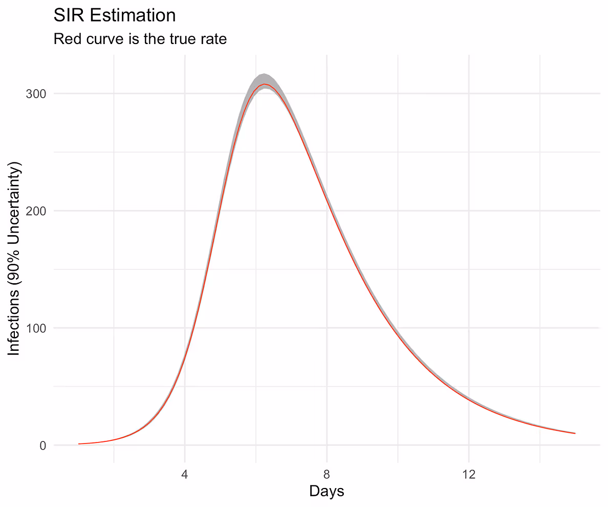
The curve follows our posterior predictive distribution.
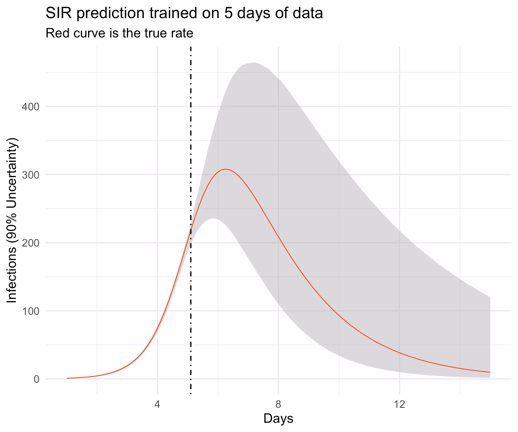
Recovering a true curve from a simulation is a good first step but I want to check if this model can predict well out-of-sample. I am not going to get into what “well” means here but will instead follow the same visual strategy as before. In particular, I will hold out some of the data from the training set and predict forward into the test set and see if we can cover the out-of-sample curve perhaps with wider uncertainty. In particular, I want to know if the model can predict the full curve before observing the peak infection rate, which in our case is slightly greater than 6 days. This requires some work in Stan’s generated quantities block. Complete code listing can be accessed here [3].
...
data {
...
  int<lower=0> n_pred;        // number of cases to predict forward
  array[n_pred] real ts_pred; // future time points
}
...
generated quantities {
  ...

  vector[n_pred] y_pred;
  vector[n_pred] lambda_pred;

  // New initial conditions
  vector[3] y_init_pred = y_hat[n_obs, ];

  // New time zero is the last observed time
  real t0_pred = ts[n_obs];

  array[n_pred] vector[3] y_hat_pred = ode_rk45(SIR,
                                                y_init_pred,
                                                t0_pred,
                                                ts_pred,
                                                theta);
  for (i in 1:n_pred) {
    lambda_pred[i] = y_hat_pred[i, 2] * n_pop;
    y_pred[i] = poisson_rng(lambda_pred[i]);
  }
}
What’s left now is to construct the new input dataset, compile the new model, sample, extract parameters, and plot the results.
pct_train <- 0.30
n_train <- floor(n * pct_train)
n_pred <- n - n_train
times_pred <- times[(n_train + 1):n]
y_train <- y[1:n_train]
data <- list(n_obs = n_train, n_pred = n_pred,
             n_pop = n_pop, y = y_train,
             t0 = 0, ts = times[1:n_train], ts_pred = times_pred)


sir_pred_mod <- cmdstan_model("sir-pred.stan")
sir_pred_fit <- sir_pred_mod$sample(
  data = data,
  seed = 1234,
  chains = 4,
  parallel_chains = 4,
  iter_warmup = 500,
  iter_sampling = 500,
  adapt_delta = 0.98
)

y_hat <- as_draws_rvars(sir_pred_fit$draws(variables = "y_hat"))
y_hat_pred <- as_draws_rvars(sir_pred_fit$draws(variables = "y_hat_pred"))

d_train <- make_df(y_hat, 0.90, data$ts, sol$I[1:n_train], n_pop)
d_pred <- make_df(y_hat_pred, 0.90, data$ts_pred, sol$I[(n_train + 1):n], n_pop)
d <- dplyr::bind_rows(d_train, d_pred)

ggplot(aes(times, obs), data = d) +
  geom_ribbon(aes(ymin = low, ymax = high),
              fill = "grey70", alpha = 1/2) +
  geom_line(color = "red", linewidth = 0.3) +
  geom_vline(xintercept = d$times[n_train], linetype = "dotdash") +
  xlab("Days") + ylab("Infections (90% Uncertainty)") +
  ggtitle("SIR prediction trained on 5 days of data",
          subtitle = "Red curve is the true rate")
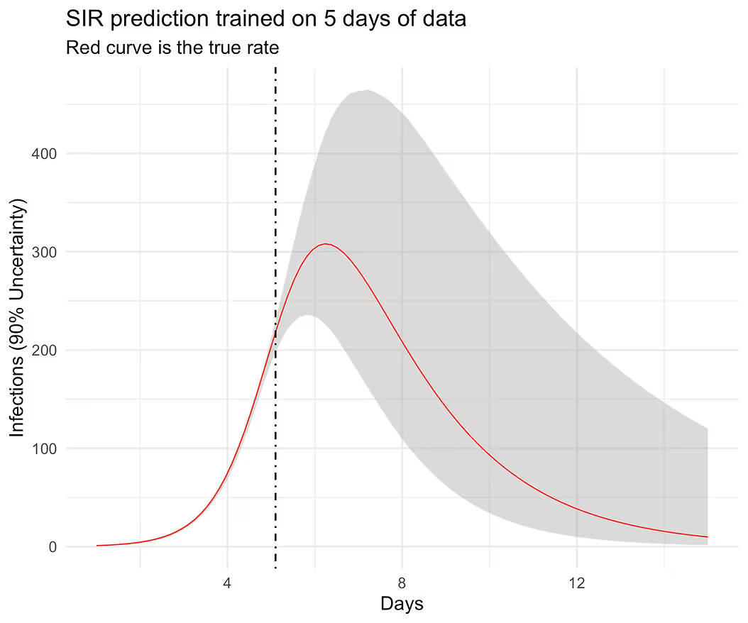
The results look believable and at this point, we can start testing the model on real data. It would be a mistake, however, to assume that this model would be good enough to work well in the wild. Complete R code listing is available here [4].
Here is a partial list of model improvements and expansions that one would likely have to do in order to model real outbreaks.
[1] Chatzilena, A., van Leeuwen, E., Ratmann, O., Baguelin, M., & Demiris, N. (2019). Contemporary statistical inference for infectious disease models using Stan. https://arxiv.org/abs/1903.00423v3
[2] public-materials/blog/SIR/sir.stan at master · generable/public-materials. GitHub. Published 2025. Accessed July 19, 2025. https://github.com/generable/public-materials/blob/master/blog/SIR/sir.stan
[3] public-materials/blog/SIR/sir-pred.stan at master · generable/public-materials. GitHub. Published 2025. Accessed July 19, 2025. https://github.com/generable/public-materials/blob/master/blog/SIR/sir-pred.stan
[4] public-materials/blog/SIR/sir.R at master · generable/public-materials. GitHub. Published 2025. Accessed July 19, 2025. https://github.com/generable/public-materials/blob/master/blog/SIR/sir.R
This is a comment related to the post above. It was submitted in a form, formatted by Make, and then approved by an admin. After getting approved, it was sent to Webflow and stored in a rich text field.
This is a comment related to the post above. It was submitted in a form, formatted by Make, and then approved by an admin. After getting approved, it was sent to Webflow and stored in a rich text field.
This is a comment related to the post above. It was submitted in a form, formatted by Make, and then approved by an admin. After getting approved, it was sent to Webflow and stored in a rich text field.
This is a comment related to the post above. It was submitted in a form, formatted by Make, and then approved by an admin. After getting approved, it was sent to Webflow and stored in a rich text field.
This is a comment related to the post above. It was submitted in a form, formatted by Make, and then approved by an admin. After getting approved, it was sent to Webflow and stored in a rich text field.
This is a comment related to the post above. It was submitted in a form, formatted by Make, and then approved by an admin. After getting approved, it was sent to Webflow and stored in a rich text field.
This is a comment related to the post above. It was submitted in a form, formatted by Make, and then approved by an admin. After getting approved, it was sent to Webflow and stored in a rich text field.
This is a comment related to the post above. It was submitted in a form, formatted by Make, and then approved by an admin. After getting approved, it was sent to Webflow and stored in a rich text field.
This is a comment related to the post above. It was submitted in a form, formatted by Make, and then approved by an admin. After getting approved, it was sent to Webflow and stored in a rich text field.
This is a comment related to the post above. It was submitted in a form, formatted by Make, and then approved by an admin. After getting approved, it was sent to Webflow and stored in a rich text field.
This is a comment related to the post above. It was submitted in a form, formatted by Make, and then approved by an admin. After getting approved, it was sent to Webflow and stored in a rich text field.
This is a comment related to the post above. It was submitted in a form, formatted by Make, and then approved by an admin. After getting approved, it was sent to Webflow and stored in a rich text field.
This is a comment related to the post above. It was submitted in a form, formatted by Make, and then approved by an admin. After getting approved, it was sent to Webflow and stored in a rich text field.
This is a comment related to the post above. It was submitted in a form, formatted by Make, and then approved by an admin. After getting approved, it was sent to Webflow and stored in a rich text field.
This is a comment related to the post above. It was submitted in a form, formatted by Make, and then approved by an admin. After getting approved, it was sent to Webflow and stored in a rich text field.
This is a comment related to the post above. It was submitted in a form, formatted by Make, and then approved by an admin. After getting approved, it was sent to Webflow and stored in a rich text field.
This is a comment related to the post above. It was submitted in a form, formatted by Make, and then approved by an admin. After getting approved, it was sent to Webflow and stored in a rich text field.
This is a comment related to the post above. It was submitted in a form, formatted by Make, and then approved by an admin. After getting approved, it was sent to Webflow and stored in a rich text field.
This is a comment related to the post above. It was submitted in a form, formatted by Make, and then approved by an admin. After getting approved, it was sent to Webflow and stored in a rich text field.
This is a comment related to the post above. It was submitted in a form, formatted by Make, and then approved by an admin. After getting approved, it was sent to Webflow and stored in a rich text field.
This is a comment related to the post above. It was submitted in a form, formatted by Make, and then approved by an admin. After getting approved, it was sent to Webflow and stored in a rich text field.
This is a comment related to the post above. It was submitted in a form, formatted by Make, and then approved by an admin. After getting approved, it was sent to Webflow and stored in a rich text field.
This is a comment related to the post above. It was submitted in a form, formatted by Make, and then approved by an admin. After getting approved, it was sent to Webflow and stored in a rich text field.
This is a comment related to the post above. It was submitted in a form, formatted by Make, and then approved by an admin. After getting approved, it was sent to Webflow and stored in a rich text field.
This is a comment related to the post above. It was submitted in a form, formatted by Make, and then approved by an admin. After getting approved, it was sent to Webflow and stored in a rich text field.
This is a comment related to the post above. It was submitted in a form, formatted by Make, and then approved by an admin. After getting approved, it was sent to Webflow and stored in a rich text field.
This is a comment related to the post above. It was submitted in a form, formatted by Make, and then approved by an admin. After getting approved, it was sent to Webflow and stored in a rich text field.

Trying to cut corners to make nonlinear PK model fitting faster

.svg)

This is a comment related to the post above. It was submitted in a form, formatted by Make, and then approved by an admin. After getting approved, it was sent to Webflow and stored in a rich text field.