


A friend asked me about how he should update his beliefs about correlation after seeing some data. In his words:
If I have two variables and I want to express that my prior is that the correlation could be anything between -1 and +1 how would I update this prior based on the observed correlation?
By observed correlation, I think he meant that he observed a realization of two random variables, and he now wants to update his beliefs about the correlation.
There is nothing special about the correlation parameter when it comes to Bayesian inference; it’s just another unknown parameter in our set of parameters $\theta$. The posterior distribution is then $p(\theta \mid y) \propto p(y \mid \theta) \cdot p(\theta)$. To make this concrete, we need to specify the form of the likelihood function $p(y \mid \theta)$. A natural one in our case is a bivariate normal distribution with the mean vector, $\mu$ and a covariance matrix, $\Sigma$. The correlation parameter can always be pulled out of $\Sigma$. Our $\theta$ is comprised of $\mu$ and $\Sigma$. The likelihood for a multivariate normal can be written as:
$$\begin{align*}
\text{MultiNormal}(y \mid \mu, \Sigma) = \frac{1}{(2\pi)^{K/2} \sqrt{|\Sigma|}}
\exp\left( -\frac{1}{2} (y - \mu)^\top \Sigma^{-1} (y - \mu) \right)
\end{align*}$$
In the above equation, $K$ is the number of output variables (2 in our case), $\Sigma$ is the 2 by 2 covariance matrix, and $\Sigma$ is the absolute value of the determinant. In the statistical notation, we usually write:
$$y \sim \text{multi_normal}(\mu, \Sigma)$$
We can work out the exact form of the posterior distribution $p(\mu, \Sigma \mid y)$ if we specify a conjugate prior on $\Sigma$. There is a well-known way of doing this, but it is both restrictive and too much work, and so we will make Stan do it for us.
My friend was interested in not being fooled by a correlation arising by chance from a small sample. In the following simulation, we will set up a covariance matrix consistent with this assumption and generate independent draws from a bivariate normal distribution.
set.seed(2)
(sigma <- matrix(c(1, 0, 0, 1), nrow = 2))

##      [,1] [,2]
## [1,]    1    0
## [2,]    0    1

(y <- mvtnorm::rmvnorm(10, mean = c(0, 0), sigma = sigma))

##              [,1]        [,2]
##  [1,] -0.89691455  0.18484918
##  [2,]  1.58784533 -1.13037567
##  [3,] -0.08025176  0.13242028
##  [4,]  0.70795473 -0.23969802
##  [5,]  1.98447394 -0.13878701
##  [6,]  0.41765075  0.98175278
##  [7,] -0.39269536 -1.03966898
##  [8,]  1.78222896 -2.31106908
##  [9,]  0.87860458  0.03580672
## [10,]  1.01282869  0.43226515

qplot(y[, 1], y[, 2])
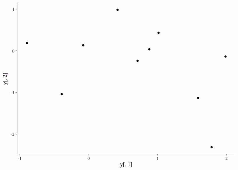
cor(y)

##            [,1]       [,2]
## [1,]  1.0000000 -0.3806624
## [2,] -0.3806624  1.0000000

cat("Sample correlation is:", round(cor(y)[1,2], 2))

## Sample correlation is: -0.38
Now that we know the sample correlation, we may be interested in quantifying the uncertainty in this correlation by computing say $\text{Pr}(\rho > −0.38)$. The simplest Stan code that I can think of that accomplishes the task is as follows.
data {
  int<lower=0> n;
  vector[2] y[n];
}
parameters {
  vector[2] mu;
  cov_matrix[2] Sigma;
}
model {
  mu ~ normal(0, 1);
  y ~ multi_normal(mu, Sigma);
}
Here, we are putting a prior on the mean vector. Priors on covariances are trickier and we are going to leave them as-is for now, which implies that the priors are uniform over all valid covariance matrices (technically positive semi-definite).
n <- nrow(y)
data <- list(y = y, n = n)
s1model <- stan_model("sigma1.stan")
s1fit <- sampling(s1model, iter = 300, data = data)
Sigma <- extract(s1fit, pars = "Sigma")$Sigma

# For each posterior draw, pull out the covariance matrix,
# convert it to correlation matrix, and pull out the correlation rho
rho1 <- apply(Sigma, 1, function(x) cov2cor(x)[1, 2])

qplot(rho1, alpha = I(1/2)) +
  geom_vline(xintercept = mean(rho1), colour = "red") +
  geom_vline(xintercept = cor(y)[1,2], colour = "blue")
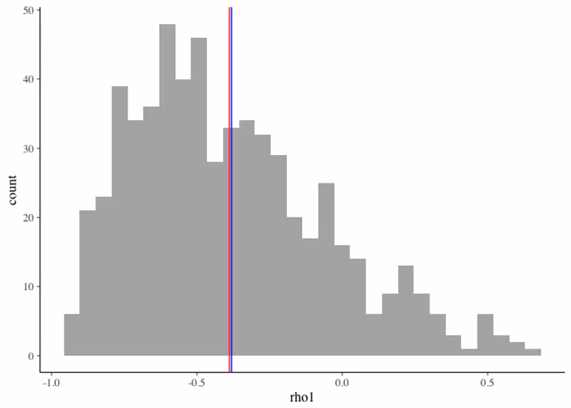
cat("Probability of the correlation exceeding -0.38:", round(mean(rho1 > -0.38), 2))

## Probability of the correlation exceeding -0.38: 0.43
The mean of the correlation under the uniform prior is very close to the point estimate from the sample, which makes sense, but the Bayes bonus, so to speak, is that we can now compute the probability that the actual correlation is greater than the point estimate and that probability is quite large, namely 0.44 which is enough to question the reality of −0.38 sample correlation.
The modern way of putting priors on the correlation matrix is to use an LKJ distribution with a parameter B. You can loosely think of ηη as a shape parameter of the Beta distribution rescaled on −1 to 1. The LKJ distribution is implemented in Stan. To see how it works, we can generate several draws from LKJ using different values of $\eta$.
We write a couple of functions in the Stan language that we want to access from R.
functions {
  real lkj_cor_lpdf(matrix y, real eta) {
    return lkj_corr_lpdf(y | eta);
  }
  matrix lkj_cor_rng(int K, real eta) {
    return lkj_corr_rng(K, eta);
  }
}
We now expose these functions to R and run simulations.
# assume lkj.stan is in the same directory
expose_stan_functions("lkj.stan")

# sample 3 x 3 correlation matrix
lkj_cor_rng(3, 1)
##            [,1]       [,2]       [,3]
## [1,]  1.0000000 -0.7097328  0.1850581
## [2,] -0.7097328  1.0000000 -0.2193609
## [3,]  0.1850581 -0.2193609  1.0000000
rho <- numeric(0)
eta <- c(0.7, 1, 2, 4)
for (i in 1:length(eta)) {
  lkj2 <- replicate(1e4, lkj_cor_rng(2, eta[i]))
  rho <- cbind(rho, apply(lkj2, 3, function(x) x[1, 2]))
}
colnames(rho) <- c("eta = 0.7", "eta = 1", "eta = 2", "eta = 4")
rho <- tidyr::gather(as.data.frame(rho))

qplot(value, alpha = I(1/3), geom = "histogram", data = rho) +
  xlab(expression(rho)) + facet_wrap(~key)
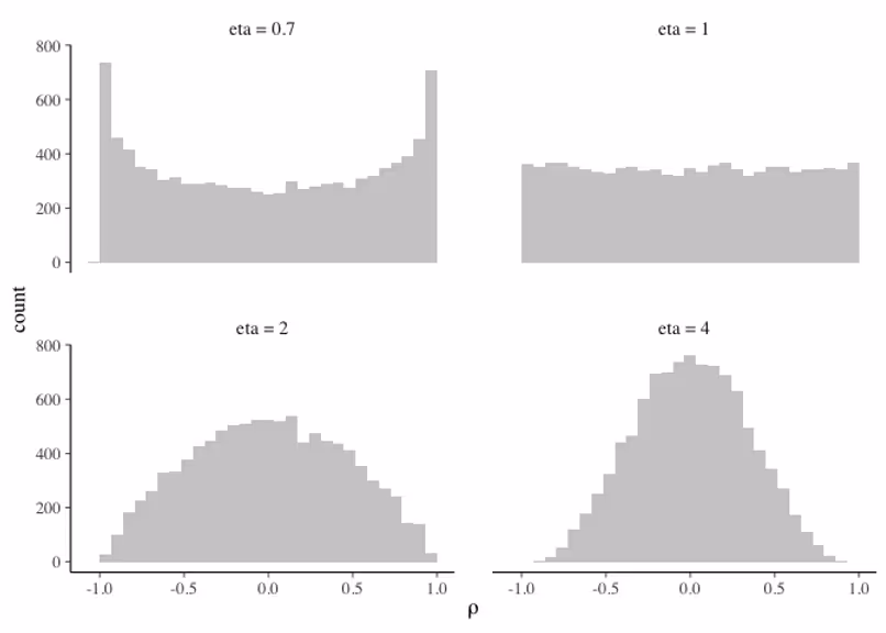
The higher the value of $\eta$, the more we believe that the correlations are close to zero. For $\eta$ less than 1, we are saying that the correlations are high in absolute value. Generally speaking, if you believe that correlations are high and positive (or high and negative), LKJ is not a great choice of prior.
Given this information, we can now construct a Stan program that would take $\eta$ as a parameter and allow us to experiment with how different prior knowledge on the correlation structure expressed through different values of $\eta$, affect the posterior inferences after seeing data.
data {
  int<lower = 1> N;    // number of observations
  int<lower = 1> J;    // number of outcome variables
  vector[J] y[N];      // observations
  real<lower = 0> eta; // shape parameter for LKJ ditribution
}
parameters {
  vector[J] mu;
  cholesky_factor_corr[J] L_Omega;
  vector<lower=0>[J] L_sigma;
}
model {
  L_Omega ~ lkj_corr_cholesky(eta);
  L_sigma ~ cauchy(0, 2.5);
  mu ~ normal(0, 1);
  y ~ multi_normal_cholesky(mu, diag_pre_multiply(L_sigma, L_Omega));
}
generated quantities {
  corr_matrix[J] Omega;
  Omega = multiply_lower_tri_self_transpose(L_Omega);
}
For the detailed description of the functions used in the above Stan code, please, consult the Stan manual. Briefly, we use Cholesky factors of the correlation matrices for computational stability. We get back the original correlation matrix scale by calling multiply_lower_tri_self_transpose() function.
We are now ready to fit this model with the original dataset and examine the posterior.
data <- list(N = nrow(y), J = 2, y = y, eta = 1) # uniform on -1 to 1
s2model <- stan_model("sigma2.stan")
s2fit <- sampling(s2model, iter = 500, data = data)
s2draws <- extract(s2fit)
Omega <- s2draws$Omega
rho2 <- apply(Omega, 2, function(x) x[,1])[, 2]

cat("Updated expected value of correlation:", round(mean(rho2), 2))
## Updated expected value of correlation: -0.28
cat("Updated standard deviation of correlation:", round(sd(rho2), 2))
## Updated standard deviation of correlation: 0.29
qplot(rho2, alpha = I(1/2)) +
  geom_vline(xintercept = mean(rho2), colour = "red") +
  geom_vline(xintercept = cor(y)[1,2], colour = "blue")
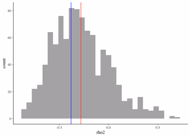
cat("Probability of the correlation exceeding -0.38:", round(mean(rho2 > -0.38), 2))

## Probability of the correlation exceeding -0.38: 0.61
The mean of the correlation parameter is now closer to zero by 0.11 and the probability of the correlation exceeding the point estimate is increased by 0.18.
If we now set a more aggressive value for $\eta$, say $\eta=4$, which is equivalent to expressing the prior knowledge that the probability of the correlation being between −0.5 and 0.5 is approximately 0.70, we can repeat the above simulation.
data <- list(N = nrow(y), J = 2, y = y, eta = 4)
s2model <- readRDS("s2model.rds")
s3fit <- sampling(s2model, iter = 500, data = data)
s3draws <- extract(s3fit)
Omega <- s3draws$Omega
rho3 <- apply(Omega, 2, function(x) x[,1])[, 2]
cat("Updated expected value of correlation:", round(mean(rho3), 2))
## Updated expected value of correlation: -0.19
cat("Updated standard deviation of correlation:", round(sd(rho3), 2))
## Updated standard deviation of correlation: 0.25
qplot(rho3, alpha = I(1/2)) +
  geom_vline(xintercept = mean(rho3), colour = "red") +
  geom_vline(xintercept = cor(y)[1,2], colour = "blue")
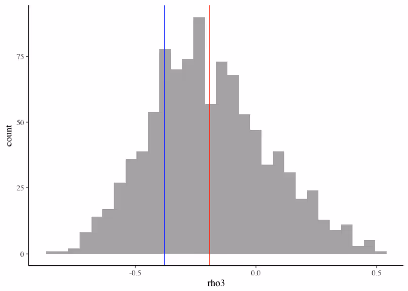
cat("Probability of the correlation exceeding -0.38:", round(mean(rho3 > -0.38), 2))

## Probability of the correlation exceeding -0.38: 0.77
To summarize, we simulated some data from two independent zero-mean normal distributions with a high (by chance) sample correlation. We showed how under the default prior the sample mean was close to the posterior mean, but we were able to quantify the uncertainty of the sample correlation. The default prior is not appropriate as we know that the correlation has to be between −1 and 1 and so we're able to construct a prior that enforced this constraint, which started to move the expected value of the correlation towards zero. Finally, we demonstrated that our prior knowledge about the correlation which could have perhaps come from previous experiments can be conveniently expressed in Stan using the LKJ distribution.
The corollary is that when working in the small data regime, which happens all the time even in big data problems, we have to be careful not to read too much into the point estimates from individual samples, but rather model the whole system, likelihood, priors and all.
This is a comment related to the post above. It was submitted in a form, formatted by Make, and then approved by an admin. After getting approved, it was sent to Webflow and stored in a rich text field.
This is a comment related to the post above. It was submitted in a form, formatted by Make, and then approved by an admin. After getting approved, it was sent to Webflow and stored in a rich text field.
This is a comment related to the post above. It was submitted in a form, formatted by Make, and then approved by an admin. After getting approved, it was sent to Webflow and stored in a rich text field.
This is a comment related to the post above. It was submitted in a form, formatted by Make, and then approved by an admin. After getting approved, it was sent to Webflow and stored in a rich text field.
This is a comment related to the post above. It was submitted in a form, formatted by Make, and then approved by an admin. After getting approved, it was sent to Webflow and stored in a rich text field.
This is a comment related to the post above. It was submitted in a form, formatted by Make, and then approved by an admin. After getting approved, it was sent to Webflow and stored in a rich text field.
This is a comment related to the post above. It was submitted in a form, formatted by Make, and then approved by an admin. After getting approved, it was sent to Webflow and stored in a rich text field.
This is a comment related to the post above. It was submitted in a form, formatted by Make, and then approved by an admin. After getting approved, it was sent to Webflow and stored in a rich text field.
This is a comment related to the post above. It was submitted in a form, formatted by Make, and then approved by an admin. After getting approved, it was sent to Webflow and stored in a rich text field.
This is a comment related to the post above. It was submitted in a form, formatted by Make, and then approved by an admin. After getting approved, it was sent to Webflow and stored in a rich text field.
This is a comment related to the post above. It was submitted in a form, formatted by Make, and then approved by an admin. After getting approved, it was sent to Webflow and stored in a rich text field.
This is a comment related to the post above. It was submitted in a form, formatted by Make, and then approved by an admin. After getting approved, it was sent to Webflow and stored in a rich text field.
This is a comment related to the post above. It was submitted in a form, formatted by Make, and then approved by an admin. After getting approved, it was sent to Webflow and stored in a rich text field.
This is a comment related to the post above. It was submitted in a form, formatted by Make, and then approved by an admin. After getting approved, it was sent to Webflow and stored in a rich text field.
This is a comment related to the post above. It was submitted in a form, formatted by Make, and then approved by an admin. After getting approved, it was sent to Webflow and stored in a rich text field.
This is a comment related to the post above. It was submitted in a form, formatted by Make, and then approved by an admin. After getting approved, it was sent to Webflow and stored in a rich text field.
This is a comment related to the post above. It was submitted in a form, formatted by Make, and then approved by an admin. After getting approved, it was sent to Webflow and stored in a rich text field.
This is a comment related to the post above. It was submitted in a form, formatted by Make, and then approved by an admin. After getting approved, it was sent to Webflow and stored in a rich text field.
This is a comment related to the post above. It was submitted in a form, formatted by Make, and then approved by an admin. After getting approved, it was sent to Webflow and stored in a rich text field.
This is a comment related to the post above. It was submitted in a form, formatted by Make, and then approved by an admin. After getting approved, it was sent to Webflow and stored in a rich text field.
This is a comment related to the post above. It was submitted in a form, formatted by Make, and then approved by an admin. After getting approved, it was sent to Webflow and stored in a rich text field.
This is a comment related to the post above. It was submitted in a form, formatted by Make, and then approved by an admin. After getting approved, it was sent to Webflow and stored in a rich text field.
This is a comment related to the post above. It was submitted in a form, formatted by Make, and then approved by an admin. After getting approved, it was sent to Webflow and stored in a rich text field.
This is a comment related to the post above. It was submitted in a form, formatted by Make, and then approved by an admin. After getting approved, it was sent to Webflow and stored in a rich text field.
This is a comment related to the post above. It was submitted in a form, formatted by Make, and then approved by an admin. After getting approved, it was sent to Webflow and stored in a rich text field.
This is a comment related to the post above. It was submitted in a form, formatted by Make, and then approved by an admin. After getting approved, it was sent to Webflow and stored in a rich text field.
This is a comment related to the post above. It was submitted in a form, formatted by Make, and then approved by an admin. After getting approved, it was sent to Webflow and stored in a rich text field.

Trying to cut corners to make nonlinear PK model fitting faster

.svg)

This is a comment related to the post above. It was submitted in a form, formatted by Make, and then approved by an admin. After getting approved, it was sent to Webflow and stored in a rich text field.