Objective is not so objective

Oct 01, 2018 | Eric Novik

Article Tags: R , Statistics , Optimization

Model selection is a difficult process, particularly in high dimensional settings, dependent observations, and sparse data regimes. In this post, I will discuss a common misconception about selecting models based on values of the objective function generated from optimization algorithms in sparse data settings. TL;DR Don’t do it.

Data Simulation

As always, I will start by simulating some data.

n <- 10
set.seed(1)
x <- rnorm(n)
a <- 1; b <- 2
y <- a + b * x + rnorm(n, sd = 3)
qplot(x, y) + geom_smooth(method = lm)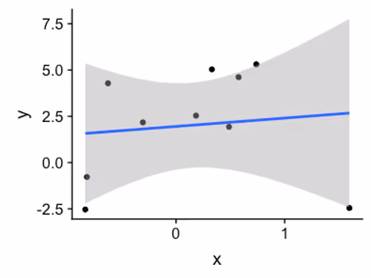

In order to fit this model with maximum likelihood, we are going to need the normal log probability density function (LPDF) and the objective function – negative of the LPDF evaluated and accumulated at each data point y. The normal PDF is defined as follows:

Taking the logs, yields:

In R, this function can be defined as follows:

normal_lpdf <- function(y, mu, sigma) {
  log(1 / (sqrt(2*pi) * sigma)) - 1/2 * ((y - mu) / sigma)^2
}

Computationally, the constants should be pre-computed, but we do not bother with this here. For sanity check, we compare to built-in R’s dnorm().

dnorm(c(0, 1), mean = 0, sd = 2, log = TRUE)
## [1] -1.612086 -1.737086

normal_lpdf(c(0, 1), mu = 0, sigma = 2)
## [1] -1.612086 -1.737086

The objective function that we will minimize is the sum of the negative log likelihood evaluated at each data point y.

# For comparison, MLE estimate using lm() function
arm::display(lm(y ~ x))

## lm(formula = y ~ x)
##             coef.est coef.se
## (Intercept) 1.95     1.01   
## x           0.45     1.35   
## ---
## n = 10, k = 2
## residual sd = 3.15, R-Squared = 0.01

# Negative log likelihood
log_lik <- function(theta, x, y) {
  ll <- -sum(normal_lpdf(y,
                         mu = theta[1] + theta[2] * x,
                         sigma = theta[3]))
  return(ll)
}

# MLE estimate using custom log likelihood
res <- optim(par = rep(1, 3), # initial values
             fn  = log_lik, 
             x   = x, 
             y   = y)
paste("Estimated value of a:", round(res$par[1], 2))
## [1] "Estimated value of a: 1.95"

paste("Estimated value of b:", round(res$par[2], 2))
## [1] "Estimated value of b: 0.45"

paste("Estimated value of sigma:", round(res$par[3], 2))
## [1] "Estimated value of sigma: 2.82"

paste("Objective function value:", round(res$value, 2))
## [1] "Objective function value: 24.56"

Now let’s see if we can decrease the value of the objective function by adding a quadratic term to the model.

arm::display(lm(y ~ x + I(x^2)))

## lm(formula = y ~ x + I(x^2))
##             coef.est coef.se
## (Intercept)  3.88     0.82  
## x            2.31     0.97  
## I(x^2)      -3.84     1.04  
## ---
## n = 10, k = 3
## residual sd = 1.96, R-Squared = 0.67

log_lik_xsqr <- function(theta, x, y) {
  ll <- -sum(normal_lpdf(y,
                      mu = theta[1] + theta[2]*x + theta[3]*(x^2),
                      sigma = theta[4]))
  return(ll)
}
res_xsqr <- optim(par = rep(1, 4), 
                  fn  = log_lik_xsqr, 
                  x   = x, 
                  y   = y)
round(res_xsqr$par, 2)

## [1]  3.88  2.31 -3.84  1.64

paste("Objective function value:", round(res_xsqr$value, 2))

## [1] "Objective function value: 19.12"

Not surprisingly, the value of the objective function is lower and R2R2 is higher.

What happens when we increase n, by say 10-fold. We still get the reduction in the objective function value but it is a lot smaller in percentage terms.